U.S. Department of Transportation
Federal Highway Administration
1200 New Jersey Avenue, SE
Washington, DC 20590
202-366-4000
Six (6) methods for establishing advisory speed are described in this chapter. The advantages and disadvantages of each method will also be discussed. The appropriate selection and application of the methods shall be considered to provide a uniform and consistent advisory speed among curves.
These methods are the most widely used or newly proposed and promising methods related to curve advisory speed determination that are accepted by transportation professionals and researchers.
The methods are all based on the premise that the selection of an advisory speed and the need for various curve warning signs should be based on the "critical" portion of the curve. The critical portion of the curve is defined as the section that has a radius and superelevation rate that combine to yield the largest side friction demand. Through this definition, the procedure is applicable to curves that have a constant radius, compound curvature, or spiral transitions.
Any of the following six (6) methods can be used to determine the curve advisory speed if used appropriately:
The Direct Method is based on field measurements of traffic speeds in the curve. The Compass Method is based on a single-pass survey technique using a digital compass, distance measuring instrument and ball-bank indicator to estimate the curve radius and deflection angle. The GPS Method is also based on a single pass survey using a GPS receiver and software to compute curve radius and deflection angle. The Design Method is useful when the radius and deflection angle are available from as built plans. The Ball-Bank Indicator Method is based on a set of field driving tests to record a ball-bank indicator reading using a ball-bank indicator and a speedometer. The Accelerometer Method is based on a set of field driving tests to measure average maximum lateral gravitational force using an electronic accelerometer device and a GPS receiver.
The six (6) methods are categorized into two general groups. The Direct Method, the Compass Method, the GPS Method, and the Design Method determine advisory speeds based on measured operating speeds or estimated operating speeds given curve geometry. The Ball-Bank Indicator Method and the Accelerometer Method determine advisory speeds based on lateral acceleration.
Regardless of which method is being used, the procedure for implementing each method consists of three steps. During the first step, measurements are taken in the field. During the second step, the measurements are used to compute the advisory speed. During the last step, the recommended advisory speed is confirmed through a field trial run. The first two steps are described for each method in the following sections. The last step is common to each method and will be described in the last section of the chapter.
As mentioned, these six (6) methods are the most widely used or newly proposed and promising methods. There may be other methods which have been used to determine curve advisory speeds, for example, Driver Comfort Speed Method and AASHTO's Geometric Design Method.
The Driver Comfort Speed Method is the oldest empirical method used for determining advisory speeds. It was defined in the 1930s as that "which causes an occupant of the vehicle to feel an outward pitch" and later refined to be "that speed at which the driver's judgment recognized incipient instability." The method is very subjective and provides inconsistent results.
The AASHTO's Geometric Design Method is based on the following equation (12) derived from the laws of mechanics and used during the traditional highway design process. The actual value of the side friction factor is different for different ranges of advisory speed and there was variation for speed and side friction relationship based on the field results (12).
V2 = 15(0.01e + f)R
where,
V = advisory speed, mph;
e = superelevation, percent;
f = side friction factor; and
R = radius of curvature, ft.
This report will not further discuss the Driver Comfort Speed Method, the AASHTO's Geometric Design Method and other non-widely used methods hereafter.
The Direct Method is based on the field measurement of vehicle speeds on the subject curve. There has been widespread discussion about how to choose the advisory speed given direct measurements of curve speed distribution and vehicle classification. The disagreement is mainly on which speed statistic and which type of vehicle should be used.
The MUTCD 2003 edition (8) recommends the advisory speed be the 85th-percentile speed of free-flowing traffic. It also stated that the 85th-percentile speed on curves approximates a 16-degree ball-bank indicator reading and is the speed at which most drivers' judgment recognizes incipient instability along a ramp or curve.
However, the MUTCD 2009 edition (3) no longer provides explicit support to use 85th-percentile free-flowing speed as the advisory speed. The manual mentions that research has shown that drivers often exceed existing posted advisory curve speeds by 7 to 10 mph. The MUTCD 2009 edition (3) references posted advisory speeds determined by ball-bank values of 16, 14, and 12 degrees to address such driver behavior.
Bonneson et al. (5) recommended that the advisory speed should be based on the average speed selected by truck drivers. This speed is 2 or 3 mph below that of passenger car drivers and thereby, represents about the 40th percentile car driver. It is rationalized that driver speed choice on sharp horizontal curves is largely influenced by safety concerns. Thus, the advisory speed should be conservative such that it informs drivers of the speed that is considered appropriate for the unfamiliar driver. Given that the speed distribution is approximately normal, the speed most commonly chosen by drivers is the average speed.
Using the direct method will allow the engineer to set the advisory speed at the speed at which drivers are driving the curve and for the type of vehicle that the curve requires.
The speed of free-flowing passenger cars should be measured at the middle of the curve in one direction of travel. A free-flowing vehicle will be at least three (3) seconds behind the previous vehicle. If a radar speed meter is used, then data collection can be discontinued after the speed of 125 cars has been measured or two hours have elapsed, whichever occurs first. If a traffic counter/classifier is used, then data collection can be discontinued after the speed of 125 cars has been measured or four hours have elapsed, whichever occurs first.
If the roadway is divided or if conditions suggest the need to consider direction of travel, the measurements should be repeated for both directions of travel. When two (2) or more curves are present, each curve should be surveyed separately in this step; however, if they are separated by a tangent section of 600 feet or less, one sign should be selected to apply to all curves.
The arithmetic average and the 85th percentile of the measured speeds should be computed for each direction of travel at each curve studied to determine the unrounded advisory speed.
Depending on the criteria chosen, the unrounded advisory speed is obtained by either calculating the 85th percentile passenger car speed or multiplying the average passenger car speed by 0.97 to obtain an estimate of the average truck speed. (Bonneson et al. (5)).
Furthermore, Bonneson et al. (5) proposed a rounding technique to determine the advisory speed. First add 1.0 mph to the unrounded advisory speed and then round the sum down to the nearest 5 mph increment to obtain the advisory speed. This technique yields a conservative estimate of the advisory speed by effectively rounding curve speeds that end in 4 or 9 up to the next higher 5 mph increment, while rounding all other speeds down. For example, applying this rounding technique to a curve speed of 54, 55, 56, 57, or 58 mph yields an advisory speed of 55 mph.
Each curve should be evaluated separately in this step; however, when two (2) or more curves are separated by a tangent of 600 feet or less, one (1) sign should apply for all curves. In this case, the Advisory Speed plaque should show the value for the curve having the lowest advisory speed in the series.
For undivided roadways, if an advisory speed is determined to be needed for one curve travel direction but not for the opposite curve travel direction, then only one direction of the curve should be posted with the advisory speed.
The Compass Method is based on a single-pass survey technique using a digital compass, distance measuring instrument and ball-bank indicator to estimate the curve geometry. Bonneson et al. (5) proposed a speed-prediction model to compute the average truck speed given the curve geometry. This speed then becomes the basis for establishing the advisory speed.
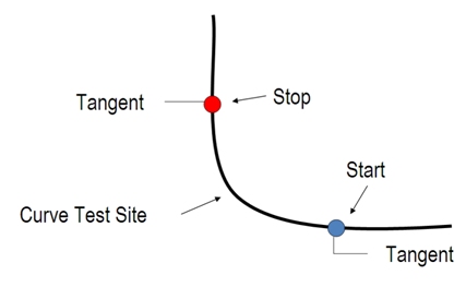
The procedure for implementing the Compass Method is based on compass heading and curve length measurements taken at the critical portion of the curve or sharpest point of the curve. When spiral transitions or compound curves are present, this critical portion of the curve is typically found in the middle third of the curve, as shown in Figure 5. If the curve is truly circular for its entire length, then measurements made in the middle third will yield the same radius estimate as those made in other portions of the curve.
Figure 5 – Location of Critical Portion of Curve
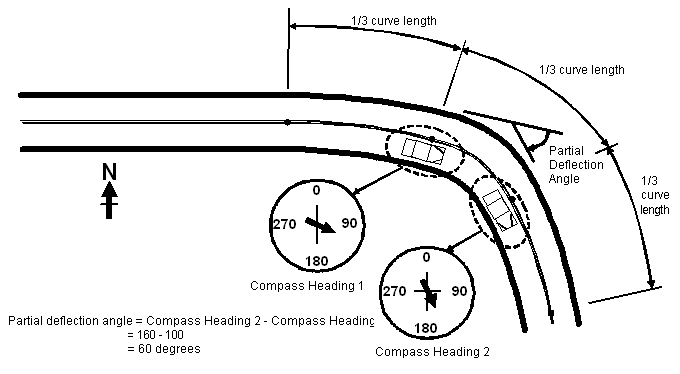
The deflection angle associated with the critical portion is referred to as the "partial deflection angle." The curve length associated with the critical portion is referred to as the "partial curve length."
To ensure reasonable accuracy in the model estimates using this method, the total curve length should be 200 ft or more and the partial curve length should be 70 ft or more. Also, the curve deflection angle should be 12 degrees or more and the partial curve deflection angle should be 4 degrees or more. A curve with a deflection angle of less than 12 degrees will rarely justify curve warning signs.
The Compass method allows the engineer to only drive the curve one time; however, this method should only be used on very low volume roads because this method requires stopping the vehicle in the travel lane.
In the first step of the procedure, the technician travels through the subject curve and makes a series of measurements. These measurements include:
These measurements may require two persons in the test vehicle, a driver and a recorder. However, with some practice or through the use of a voice recorder, it is possible that the driver can also serve as the recorder such that a second person is not needed. The next two subsections describe the procedure for making the aforementioned field measurements.
If the road is divided or if conditions suggest the need for separate consideration of each travel direction, the measurements should be repeated for the opposing direction of travel. If multiple curves are present, each curve should be evaluated separately in this step; however, when two (2) or more curves are separated by a tangent of 600 feet or less, one (1) sign should apply for all curves.
The test vehicle will need to be equipped with the following three devices:
The digital compass heading calculation should be based on global positioning system (GPS) technology with a position-accuracy of 10 feet or less 95 percent of the time and a position update interval of one (1) second or less. It must also have a precision of 1 degree (i.e., provide readings to the nearest whole degree).
The compass should be installed in the vehicle in a location that is easily accessed and in the recorder's field of view. The type of mounting apparatus needed may vary; however, the compass should be firmly mounted so that it cannot move while the test vehicle is in motion.
The DMI is used to measure the length of the curve. It should have a precision of 1 ft (i.e., provide readings to the nearest whole foot). The DMI can also be used to: (1) locate a specific curve (in terms of travel distance from a known reference point), and (2) verify the accuracy of the test vehicle's speedometer. The DMI can be mounted in the vehicle, but should be removable such that it can be hand-held during the test run.
The ball-bank indicator must have a precision of at least one (1) degree (i.e., provide readings to the nearest whole degree). Indicators with less precision (e.g., 5 degree increments) cannot be used with this method. The indicator should be installed along the center of the vehicle in a location that is easily accessed and in the recorder's field of view. The center of the dash is the recommended position because it allows the driver to observe both the road and the indicator while traversing the curve. The type of mounting apparatus needed may vary; however, the ball-bank indicator should be firmly mounted so that it cannot move while the test vehicle is in motion.
To ensure proper operation of the devices, it is important that the following steps are taken before conducting the test runs:
The instruction manual should be consulted for specific details about the calibration process for the DMI and the ball-bank indicator.
The following task sequence describes the field measurement procedure as it would be used to evaluate one direction of travel through the subject curve. Measurement error and possible differences in superelevation rate between the two directions of travel typically justify repeating this procedure for the opposing direction. Only one test run should be required in each direction.
The value shown on the DMI is the partial curve length. With some practice, it may be possible to complete the two tasks listed above while the vehicle is moving slowly (i.e., 15 mph or less). However, if the measurements are taken while the vehicle is moving, is imperative that they represent the heading and length for the same exact point on the roadway. Error will be introduced if the heading is noted at one location and then the length is measured at another location.
Safety should be considered before stopping the vehicle in the travel lane on a curve or if moving slowly through the curve. Additional maintenance of traffic may be required to perform this step safely.
During this step, the field measurements are used to determine the appropriate advisory speed for a specified travel direction through the subject curve. The calculations are then repeated to obtain the advisory speed for a different curve or for the opposing direction of travel through the same curve.
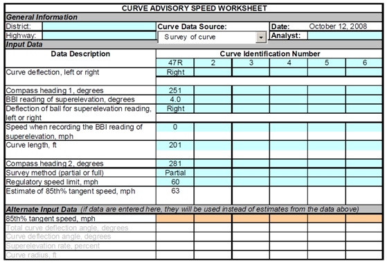
Initially, the data collected are entered in the Analysis worksheet of the Curve Advisory Speed (CAS) software. The entry of data for example curve "47R" is shown in Figure 6. The measurements taken at this curve are shown in the column headed by the curve's identification number. The curve deflected to the right, relative to the direction of travel during curve measurement.
The compass heading at the first "1/3 point" was 251 degrees. A ball-bank indicator reading of 4.0 degrees was noted at this point. The ball deflected to the right of the "0.0 degrees" tick mark. This direction indicates that a positive (i.e., beneficial) superelevation is provided along the curve. The vehicle was stopped for these two measurements, so the vehicle speed was input as "0 mph" when the ball-bank indicator was read.
A curve length of 201 ft was measured at the "2/3 point." The compass heading at this point was 281 degrees. Finally, the regulatory speed limit of 60 mph is entered into the spreadsheet.
Figure 6 – Curve Advisory Speed (CAS) Software Input Data
The speed limit is used to estimate the 85th percentile speed on the highway tangents in the vicinity of the curve. If the 85th percentile tangent speed is known, then it can be directly entered in the first row of the Alternate Input Data section of the worksheet (i.e., the fifth row from the bottom, in Figure 6). If a value is entered in the Alternate Input Data section, then it will be used instead of the value estimated using the field measurements entered in the Input Data section. This priority is extended to the direct entry of 85th percentile tangent speed, curve deflection angle, superelevation rate, curve radius, or any combination of these data.
The advisory speed is computed using the estimated (or directly input) curve radius, deflection angle, and superelevation rate. A curve-speed prediction model is used for this purpose. The estimate obtained from this model represents the "unrounded advisory speed" and is shown in the second row from the bottom of Figure 7. The advisory speed is computed by first adding 1.0 mph to the unrounded speed and then rounding the sum down to the nearest 5 mph increment. The rationale for this rounding technique is discussed in the Direct Method Section 3.2.2. The rounded advisory speed is shown in the last row of Figure 7.
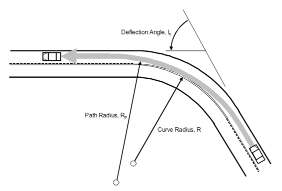
It should be noted that the computed advisory speed is based on the estimated radius of the vehicle's travel path, as opposed to that of the curve. When traveling through a curve, drivers shift their vehicle laterally in the traffic lane, such that the curve is flattened slightly. This behavior allows them to limit the speed reduction required by the curve. The difference between the radius of the curve and the travel path radius is shown in Figure 8. The estimated path radius for the subject curve is listed in the Advisory Speed section of the analysis worksheet, as shown in Figure 8. It will always equal or exceed that of the curve radius. The path radius will be notably larger than the curve radius on curves with a smaller deflection angle.
Figure 7 – Curve Advisory Speed (CAS) Software Advisory Speed Calculation
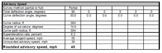
Figure 8 – Effect of Lateral Shift on Travel Path Radius
In this step, when two or more curves are present, each curve should be evaluated separately; however, if they are separated by a tangent section of 600 ft or less, one sign should apply for all curves. The Advisory Speed plaque should show the value for the curve that has the lowest advisory speed in the series.
For undivided roadways, if an advisory speed is determined to be needed for one curve travel direction but not for the opposite curve travel direction, then only one direction of the curve should be posted with the advisory speed.
The GPS Method is based on the field measurement of curve geometry. The geometric data are then used with a speed prediction model to compute the average speed of trucks. This speed then becomes the basis for establishing the advisory speed.
To ensure reasonable accuracy in the model estimates using this method, the total curve deflection angle should be 6 degrees or more. Curves with a smaller deflection angle rarely justify curve warning signs or an advisory speed plaque.
The GPS method allows the engineer to only drive the curve one time; however, this method requires driving the curve at a low speed.
The equipment used includes the following:
The GPS receiver is used to estimate curve radius and deflection angle. The electronic ball bank indicator, which is used to estimate superelevation rate, is optional. If an electronic ball-bank indicator is not used, then superelevation rate will need to be estimated using other means. The computer is used to run the Texas Roadway Analysis and Measurement Software (TRAMS) program. This program is designed to monitor the GPS receiver and the electronic ball bank indicator while the test vehicle is driven along the curve. After the curve is traversed, TRAMS calculates curve radius and superelevation rate from the data streams. Advisory speed and traffic control device selection guidelines can be determined using the radius and superelevation rate estimates with the Curve Advisory Speed (CAS) software.
The following activities must be completed the first time TRAMS is installed on the computer. More details are provided in the TRAMS Installation Manual and are available from TTI.
The following activities must be completed prior to using the equipment to establish the advisory speed for one or more curves.
Figure 9 – GPS Method Equipment Setup in Test Vehicle
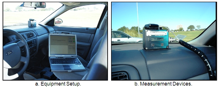
Figure 10 – Texas Roadway Analysis and Measurement Software (TRAMS) Main Panel
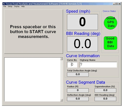
Before beginning a test run, the curve number and highway name should be entered in their respective fields provided on the main panel (see Figure 10).
If the roadway is divided or if conditions suggest the need for consideration of each direction of travel, the measurements should be repeated for the opposing direction of travel. When two (2) or more curves are separated by a tangent of 600 ft or less, one sign should apply to all curves even though each curve should be surveyed separately in this step.
If the 85th percentile tangent speed is not known, the regulatory speed limit on the roadway where the curve is located should be noted. The speed limit can subsequently be used in Curve Advisory Speed (CAS) software to estimate the 85th percentile tangent speed.
The following rules of thumb should be considered when selecting the test run speed:
In general, slower test run speeds improve measurement accuracy by minimizing tire slip and allowing the driver to track the curve more accurately.
The following task sequence describes the field measurement procedure as it would be used to evaluate one direction of travel through the subject curve. Measurement error and possible differences in superelevation rate between the two directions of travel typically justify repeating this procedure for the opposing direction. Only one test run should be required per direction.
When asked whether a curve report file should be saved, "yes" can be indicated by pressing Enter (or clicking on the Yes button). Alternatively, "No" can be indicated if it is believed that the curve was not accurately measured during the test run (e.g., the driver did not accurately track the curve, or the data recording was not started and stopped at the appropriate times). CAUTION: If the curve has the same number as a curve that was previously evaluated, the new file will overwrite the file from the previous curve.
At the conclusion of the test run, the 95th percentile error range for superelevation rate is provided in the curve report file. It can be checked to confirm that the estimated value is reasonably precise based on field observations. If this range exceeds 3 percent, the test run should be repeated at a lower speed. If the aforementioned test run speed rules of thumb (section 3.4.1.5) were followed, this check should not be needed.
The curve report file can be accessed from the main panel by selecting File, Open Curve Report, and selecting the appropriate "log" file. The file will be named "Curve XX Rpt.Log," where XX will be replaced by the curve number entered on the main panel before the start of the test run. Once the file is selected, selecting Open will open the file in a text editor.
Two options are available for determining the advisory speed. One option is based on a review of the survey data in the field. The second option is based on a review of the survey data in the office, following the survey of all curves of interest.
When multiple curves are present in succession, each curve should be evaluated separately; however, when two or more curves are separated by a tangent of 600 ft or less, one sign should apply for all curves. In this case, the Advisory Speed plaque should show the value for the curve that has the lowest advisory speed in the series.
For undivided roadways, if an advisory speed is determined to be needed for one curve travel direction but not for the opposite curve travel direction, then only one direction of the curve should be posted with the advisory speed.
Option 1: In Field Determination
Figure 11 – Import TRAMS Data
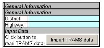
The imported data from TRAMS are always placed in the same CAS column (i.e., column F). Therefore, if the analyst wants to save any data in this column, then he or she should copy and paste the data to another column in CAS software (or another spreadsheet) and save the file.
Option 2: In Office Determination
This option is performed back in the office. The curve report file for each curve is opened in text editor and printed by selecting File, Print. There is one report for each unique curve number entered in TRAMS. The data on the report can then be typed into CAS software and the appropriate advisory speed can be determined. Instructions for opening a curve report file were provided in Section 3.4.1.8.
The Design Method is based on the use of curve geometry data obtained from files or as built plans. This method is suitable for evaluating newly constructed or reconstructed curves because the needed data are available from the construction plans. However, data for the design method may not be readily available for most curves.
The appropriate files must be consulted to obtain the radius, deflection angle, and superelevation rate for the curve. If the curve is circular, the "total curve deflection angle" is equivalent to the "curve deflection angle," as used in CAS software. The total curve deflection angle equals the deflection angle of the two intersecting tangents.
If spiral transition curves are included in the design, the radius and superelevation rate data for the central circular curve should be obtained. The total curve deflection angle is the same as defined in the previous paragraph. The curve deflection angle represents the deflection angle of the central circular curve, defined previously as the partial deflection angle.
If compound curvature is used in the design, the radius and superelevation rate data for the sharpest component curve should be obtained. The total curve deflection angle is the same as defined in the first paragraph. The curve deflection angle represents the deflection angle of the sharpest component curve.
If the road is divided or if conditions suggest the need for separate consideration of each curve travel direction, the aforementioned data for both directions of travel should be obtained. Although data for each curve should be obtained separately in this step, when two or more curves are separated by a tangent of 600 ft or less, one sign should apply for all curves.
The data obtained are entered in CAS software in the section titled Alternate Input Data. Note: the drop-down list at the top of the spreadsheet should be set to "Known curve geometry". If a reasonable estimate of the 85th percentile tangent speed is not available, the speed limit can be used in CAS software to estimate the 85th percentile tangent speed.
Each curve should be evaluated separately in this step, but when two or more curves are separated by a tangent of 600 ft or less, one sign should apply for all curves. In this case, the Advisory Speed plaque should show the lowest advisory speed for the series of curves.
For undivided roadways, if an advisory speed is determined to be needed for one curve travel direction but not for the opposite curve travel direction, then only one direction of the curve should be posted with the advisory speed.
The Ball-Bank Indicator Method is based on a set of field driving tests to record ball-bank indicator reading using a ball-bank indicator and a speedometer. There are varied criteria for establishing the curve advisory speed based on ball-bank indicator readings.
The AASHTO's Geometric Design of Highways and Streets (2004) states that curve speeds that do not cause "driver discomfort" corresponding to ball-bank readings of 14-degree for speeds of 20 mph or less, 12-degree for speeds of 25 to 30 mph, and 10-degree for speeds of 35 mph or more. It notes that these readings are consistent with side friction factors of 0.21, 0.18, and 0.15, respectively.
The MUTCD 2003 edition indicates that the advisory speed may be the speed corresponding to a 16-degree ball-bank indicator reading. However, the MUTCD 2009 edition (3) modified the criteria as following:
The manual mentions that research has shown that drivers often exceed existing posted advisory curve speeds by 7 to 10 mph. The MUTCD 2009 edition (3) references posted advisory speeds determined by ball-bank values of 16, 14, and 12 degrees to address such driver behavior.
Ball-Bank Indicator Method determines the advisory speeds in the field using a vehicle equipped with a ball-bank indicator and an accurate speedometer. The speedometer should be check using a calibrated radar gun or other method. The simplicity of construction and operation of this device has led to its widespread acceptance as a guide to determine advisory speeds for changes in horizontal alignment. Figure 12 shows a typical ball-bank indicator.
Figure 12 – Ball-Bank Indicator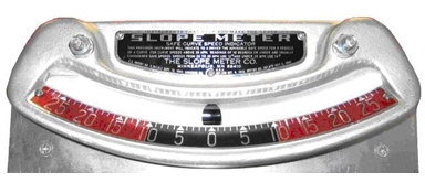
The ball-bank indicator consists of a curved glass tube which is filled with a liquid. A weighted ball floats in the glass tube. The ball-bank indicator is mounted in a vehicle, and as the vehicle travels around a curve, the ball floats outward in the curved glass tube. The movement of the ball is measured in degrees of deflection, and this reading is indicative of the combined effect of superelevation, lateral (centripetal) acceleration, and vehicle body roll. The amount of body roll varies somewhat for different types of vehicles, and may affect the ball-bank reading by up to one degree, but generally is insignificant if a standard passenger car is used for the test. Therefore, when using this technique, it is best to use a typical passenger car rather than a pickup truck, van, or sports utility vehicle. Also, the ball-bank indicator test is normally a two-person operation, one person to drive and the other to record curve data and the ball-bank readings, especially if advisory speeds are being determined for a series of curves.
The Ball-Bank Indicator method requires two people in the vehicle and multiple runs through the curve to get the correct advisory speed. In addition, reading the ball-bank indicator to determine the maximum degree of lean can be subjective.
To ensure proper results, it is critical that the following steps be taken before starting test runs with the ball-bank indicator:
The vehicle speedometer is calibrated to ensure proper and consistent test results. This can be done by checking the vehicle speed with a radar or laser speed meter, or by timing the vehicle over a measured distance (such as milepost spacing). Alternatively, a moving radar unit can be used to measure speed while conducting the ball-bank test runs rather than relying on the vehicle's speedometer.
The ball-bank indicator must be mounted in the vehicle so that it displays a 0-degree reading when the vehicle is stopped on a level surface. The positioning of the ball-bank indicator is checked before starting any test. This can be done by stopping the car so that its wheels straddle the centerline of a two-lane highway on a tangent alignment. In this position, the vehicle is essentially level, and the ball-bank indicator gives a reading of 0-degree. It is essential that the driver and recorder be in the same position in the vehicle when the ball-bank indicator is set to a 0-degree reading as they will be when the test runs are made because a shift in the load in the vehicle can affect the ball-bank indicator reading.Starting with a relatively low speed, the vehicle is driven through the curve at a constant speed following the curve alignment as closely as possible, and the reading on the ball-bank indicator is noted. On each test run, the driver must reach the test speed at a distance of at least ¼ mile in advance of the beginning of the curve, and maintain the same speed throughout the length of the curve. The path of the car must be maintained as nearly as possible in the center of the innermost lane (the lane closest to the inside edge of the curve) in the direction of travel. If there is more than one lane in the direction of travel, and these lanes have differing superelevation rates, the lane with the lowest amount of superelevation should be used. Because it is often difficult to drive the exact radius of the curve and keep the vehicle at a constant speed, it is suggested that at least three test runs in each direction be made to more accurately determine the ball-bank reading for any given speed. On each test run, the recorder carefully observes the position of the ball throughout the length of the curve and records the deflection reading that occurs when the vehicle is as nearly as possible driving the exact radius of the curve.
If the reading on the ball-bank indicator for a test run does not exceed the criteria stated in the MUTCD 2009 edition (3) (see Section 3.6, above), then the speed of the vehicle is increased by 5 mph and the test is repeated. The vehicle speed is repeatedly increased in 5 mph increments until the ball-bank indicator reading exceeds the acceptable maximum.
The curve advisory speed is set at the highest test speed that does not result in a ball-bank indicator reading greater than an acceptable level.
For example, a series of test runs for a curve were started at 25 mph, with ball-bank indicator reading of about 6-degree. This is well below the suggested criteria of 14-degree for a speed of 25 mph. The speeds of the test runs were increased in five mile an hour increments until the speed of 35 mph gave readings of 10-degree to 12-degree. These are the highest readings attained without exceeding the suggested criteria of 12-degree for a speed of 35 mph or more, because the speed of 40 mph gave the readings of 13-degree to 15-degree. Therefore, this field measurement would result in posting an advisory speed of 35 mph for this curve.
An accelerometer is an electronic device which can measure the lateral (centripetal) acceleration experienced by a vehicle as it travels around a curve. The Accelerometer Method can be used as an alternative to the Ball-Bank Indicator Method to establish the advisory speed (AASHTO's 2004 Green Book (12), and MUTCD 2009 edition (3)).
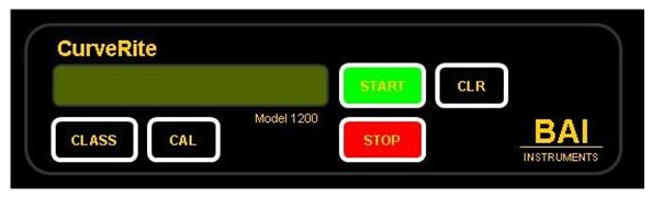
The accelerometer is mounted on a level surface in a standard passenger vehicle such as on the windshield or along the floor centerline. An example of a commercially available unit is CurveRite 1200 shown in Figure 13. The CurveRite unit is equipped with a high-grade accelerometer and GPS that measures the lateral gravitational force that the vehicle encounters and the speed in which the average maximum lateral gravitational force was encountered.
Figure 13 – CurveRite Front Panel
Similar to the ball-bank indicator study procedure, the vehicle is driven through a curve at a constant speed following the radius of the curve as closely as possible. The advisory speed of the curve is set at the highest speed that can be driven without exceeding a specified, comfortable lateral acceleration. The accelerometer does not require a second person to act as recorder because the data are stored for later recording, or the data can be transferred to a computer back at the office.
Under normal conditions, the suggested advisory speed for comfort in a passenger vehicle is when the average lateral gravitational force displayed on the device is 0.28 g (ft/sec2), Brudis & Associates, Inc. (13). A measurement of 0.26 g (ft/sec2) to 0.30 g (ft/sec2) is considered an acceptable range for establishing advisory speeds. The operator should not conduct a test run through any curve in excess of 0.40 g (ft/sec2).
The Accelerometer method requires only one person in the vehicle and multiple runs through the curve to get the correct advisory speed. The accelerometer provides the maximum lateral gravitational force and the speed at which that force occurred for each run.
After a thorough site assessment, the operator may begin conducting tests at the curve site. The operator should note any unique characteristics of the curve such as intersections, adequate sight distances etc. In order to reflect the worst condition of the curve, test runs should be made on the inside of the curve or the travel lane with the shortest radius. It is important to maintain a smooth, uniform path throughout the curve; any sudden movement will cause an inaccurate measurement. It is important to remember to drive at a constant speed, stay on a steady path and maintain a constant speed based on the speedometer within the vehicle (note: Cruise control cannot be used during the test run to avoid fluctuation due to a change in vertical grade). The predetermined speed must be held constant, if constant speed is not maintained, repeat the run and record both results.
Select either a compact, mid-size, or sports utility vehicle in good working condition to prepare for the installation of the meter. The suspension of the vehicle should not have been modified. The vehicle must sit level upon its suspension and the tires should be evenly inflated. Before test runs, secure accelerometer, connect GPS, prepare power connection and calibrate the CurveRite according to the instructional manual.
To obtain adequate measurements, the operator must drive a CurveRite equipped test vehicle through the same curve. After each pass the operator will increase the test vehicle speed by five mph increments. The CurveRite consistently records the average maximum lateral gravitational force (g-force) of each pass through the curve. The initial test vehicle speed selected should be 5 to 10 mph below the existing posted advisory speed. The speed of the vehicle is then increased in 5 mph increments in order to obtain a lateral g-force measurement above the recommended value of 0.28 g. The vehicle operator should stop increasing curve speeds when the test measurements exceed 0.40 g. Test runs should be conducted by following the steps:
Figure 14 – CurveRite Measurement
The curve advisory speed is set at the highest test speed that does not result in CurveRite reading greater than 0.28 g (ft/sec2).
For example, a series of test runs for a curve were started at 25 mph, then 30 mph, 35 mph, and 40 mph, with CurveRite reading of 0.22 g, 0.26 g, 0.28 g, and 0.29 g, respectively. 35 mph is the highest testing speed without exceeding the suggested criteria of 0.28 g. Therefore, this field measurement would result in posting an advisory speed of 35 mph for this curve.
This procedure is to evaluate the appropriateness of the advisory speed determined. The field evaluation of curve conditions includes consideration of the following factors:
The unexpected geometric features noted in the third bullet may include:
A test run shall be conducted through the curve while traveling at the advisory speed determined in the previous description for each method. The engineer may choose to adjust the advisory speed or modify the warning sign layout based on consideration of the aforementioned factors.
For undivided roadways, if an advisory speed is determined to be needed for one curve travel direction but not for the opposite curve travel direction, then only one direction of the curve should be posted with the advisory speed.
A series of four workshops and one webinar were held across the country on establishing advisory curve speeds. The workshops were held in Maine, Virginia, Illinois and California. Discussions and comments that came up during the workshops included the following:
In this chapter, the six (6) methods for establishing advisory curve speeds were introduced; and methodological procedures, including required equipments, software, installation and setup, and testing steps in the field were described. All methods can be used with the Curve Advisory Speed (CAS) software. The advisory speed is then determined based on the field measurements or known information and adjusted based on field confirmation and judgment.
The Direct Method is based on the field measurement of curve speeds under free-flow conditions. The devices used to record speeds are usually a radar speed meter and/or a traffic counter/classifier, both of which are commonly available devices to most traffic agencies. However, the traffic agencies do not have unanimous agreement regarding how best to determine the advisory speed given the distribution of curve speed and vehicle classification. The disagreement involves whether to use 85th percentile, average, or median speeds, as well as whether to use speeds of passenger cars, trucks, or all vehicles. Setting advisory speeds at 85th percentile speeds has been an accepted and common practice in the past, while also supported by the MUTCD 2003 edition, but is no longer a preferred approach in the MUTCD 2009 edition (3). Bonneson et al. (5) recommended using average truck speeds to determine advisory speeds.
The Compass Method is based on a single-pass survey technique using a digital compass, distance measuring instrument and ball-bank indicator to estimate the curve radius and deflection angle. The GPS Method is also based on a single pass survey using a GPS receiver and software to compute curve radius and deflection angle. The Design Method is useful when the radius and deflection angle are available from as built plans. The three methods were based on the TTI proposed curve speed prediction model which correlates the curve speed with the curve geometry. An Excel spreadsheet program Curve Advisory Speed (CAS) software was developed by TTI and hereafter enhanced to provide a means to calculate advisory speeds given curve geometry. The default model in the program is setting advisory speeds at average truck speed. The parameters in the program can be customized to setting advisory speeds at 85th percentile speeds of trucks and/or passenger cars.
The Ball-Bank Indicator Method is based on field driving tests to record ball-bank indicator readings using a ball-bank indicator and a speedometer. The simplicity of construction and operation of this device has led to its widespread acceptance as a guide to determine advisory speeds for changes in horizontal alignment; however, there are varied criteria for establishing the curve advisory speed based on ball-bank indicator readings. The AASHTO Green Book 2004 (12) recommends setting advisory speeds based on 14-degree for speeds of 20 mph or less, 12-degree for speeds of 25 to 30 mph, and 10-degree for speeds of 35 mph or more. The MUTCD 2009 edition (3) recommends the criteria of 16-degree, 14-degree, and 12-degree for the same range of speeds as in the AASHTO's. The manual mentions that research has shown that drivers often exceed existing posted advisory curve speeds by 7 to 10 mph. The MUTCD 2009 edition (3) references posted advisory speeds determined by ball-bank values of 16, 14, and 12 degrees to address such driver behavior.
The Accelerometer Method is based on field driving tests that measure average lateral gravitational force using an electronic accelerometer device and a speedometer. It is an alternative to the Ball-Bank Indicator Method that is used to establish the advisory speed. CurveRite is a currently commercially available unit that can collect the required measurements. Unlike the Ball-Bank Indicator Method which needs two (2) people to collect the data, CurveRite requires only one (1) person to run the tests. Under normal conditions, the suggested advisory speed to maintain comfort in a passenger vehicle is when the average lateral gravitational force displayed on the device is 0.28 g (ft/sec2).
The following table (Table 1) summarizes the advantages and disadvantages for the six (6) methods discussed in this report.
| Method | Advantages | Disadvantages |
|---|---|---|
| Direct |
|
|
| Compass |
|
|
| GPS |
|
|
| Design |
|
|
| BBI |
|
|
| Accelerometer |
|
|
No matter which method is chosen for establishing the advisory speed, the enhanced Excel spreadsheet program Curve Advisory Speed (CAS) software also has the capability to recommend the appropriate warning signs in advance of and/or at curves according to the MUTCD 2009 edition (3) criteria, given the advisory speed, the posted speed limit along the tangent section and other geometric features.

