2.0 Planning: Problem Identification

< Previous

Table of Contents

Next >

Unit 2 addresses the problem identification step in the HSIP planning process.  It begins by clarifying the difference between nominal safety (based on design standards) and substantive safety (based on roadway safety performance).  Since the state HSIP is data driven, quality data and data collection processes are important aspects of the problem identification process.  This unit identifies potential data challenges and methods for addressing them.  It also outlines how to apply safety data in the network screening process to identify safety issues to address with systemic improvements or sites with potential for safety improvement.  Several alternative methods are presented to identify locations or roadway segments with potential for safety improvement. 

2.1 Nominal and Substantive Safety

Roadway safety can be characterized as nominal or substantive.  Nominal safety is based on design standards, while substantive safety is based on roadway safety performance.

Nominal Safety

Nominal safety refers to whether or not a design (or design element) meets minimum design criteria based on national or state standards and guidance documents such as the AASHTO Green Book and the MUTCD.  If a roadway meets minimum design criteria, it can be characterized as nominally safe.  However, nominal safety does not characterize the actual or expected safety of a roadway.

Substantive Safety

Conversely, substantive safety refers to the actual or expected safety on a roadway.  Substantive safety may be quantified in terms of:

• Crash frequency (number of crashes for a given road segment or intersection over a specified time period);
• Crash rate (normalized to account for exposure);
• Crash type; and/or
• Crash severity (i.e., fatality, injury, or property damage only).

A roadway can be characterized by its safety performance relative to an expected value for the facility type; this could include regional, state, or national averages, or some other measurement.  It is important to compare a road to similar roads because the expected safety performance of the road is strongly related to its context (e.g., traffic volume, location, design type, terrain, etc.).  If the roadway in question has a significantly higher incidence or severity of crashes than other roads of its kind, it may have a substantive safety problem.  Also, unusual crash patterns, such as more angle or nighttime crashes than on other facilities with similar characteristics, may indicate a problem, such as insufficient signage or lighting.

Relating Nominal and Substantive Safety

A direct correlation does not exist between nominal and substantive safety.  A roadway may be characterized as nominally safe (meets minimum design criteria), while having higher than expected crash experience.  Similarly a roadway not meeting minimum design criteria may still function at a high level of substantive safety.

Substantive safety requires an evidence-based approach to estimate the expected safety of a roadway through data and analysis rather than focusing solely on standards.  This requirement creates a need for quality data and data systems.

Since the state HSIP is data-driven, quality data and data collection processes are important.  The next section focuses on the data collection process and sources, data issues and challenges, and methods for overcoming those challenges.

2.2 Data Collection

Crash data systems are used by local, state, and Federal agencies as the basis of road safety and injury prevention programs.  However, other data systems are important for managing road safety, including roadway, emergency medical services (EMS), hospital outcome, and enforcement data (e.g., citations, convictions, and sentencing outcomes).  The data are used by transportation design, operations, and maintenance personnel as well as safety professionals in enforcement, education, emergency medical services, and public health communities to identify problem areas, select countermeasures, and monitor countermeasure impact.
This section outlines the data collection process as well as current and potential deficiencies in the data.  It concludes with methods for addressing data challenges.

Data Collection and Management Methods

The path of crash data from the point of collection to analysis is complicated and varies from state to state and even within local governments.  Crash data are originally collected either by state or local law enforcement officers in the field or are self-reported by vehicle owners.

When crashes occur, state or local law enforcement is called to the scene.  The officer completes a crash report (commonly referred to as police accident reports or PAR) documenting the specifics of the crash.  The contents of the crash report are predetermined by the local or state government.  The report documents information related to the location of the crash, vehicles involved, and drivers and passengers in the vehicles.  (NHTSA maintains a catalog of state crash forms.)

While some states are collecting crash reports electronically, most data are entered into a state crash database manually or through a scanning process.  Typically the state agency responsible for maintaining the crash database uses the crash report to identify and record the crash location.  Reports with missing or unclear information are handled manually to determine if the information can be recovered.  The time from which crash data are collected until they are available for analysis varies depending on the type of crash reporting system, and state and local government database capabilities.  While some states are close to providing data with a very short turnaround (e.g., real time to a month); others may not have complete data available for up to two years.\

The state crash database usually is maintained by the state DOT, state law enforcement agency or the Department of Motor Vehicles (DMV).  Various programs and departments, such as local governments, metropolitan planning organizations (MPO), advocacy groups, and private consultants request state crash data to conduct various planning activities and analyze projects.  The agency maintaining the database generally fills the requests by providing raw or filtered datasets.

Additional Data Sources

In addition to state-level crash data systems, agencies frequently use information from the following national databases:  Fatality Analysis Reporting Systems (FARS), the Motor Carriers Management Information System (MCMIS), and in some states, the Crash Outcome Data Evaluation System (CODES).

Crashes involving fatalities are reported to NHTSA and further investigated for inclusion in FARS, which contains annual data on a census of fatal traffic crashes within the 50 states, the District of Columbia, and Puerto Rico.  According to NHTSA, “…to be included in FARS, a crash must involve a motor vehicle traveling on a traffic way customarily open to the public, and must result in the death of an occupant of a vehicle or a nonmotorist within 30 days of the crash.”  FARS data are available annually back to 1975.  FARS contains more than 100 data elements related to the driver, vehicle, involved persons, and the crash itself.  The FARS web site allows users to run national or state-specific reports on multiple factors related to trends, crashes, vehicles, people, and states.  It also provides a query tool which allows users to download raw data for individual analysis.  FARS is a widely used information source for research and program evaluation focusing on fatal crashes.

NHTSA’s State Traffic Safety Information (STSI) web site provides quick and easy access to state traffic facts, including:  fatalities for years 2004-2008; by the various performance measures; by county; and economic impact of motor vehicle crashes.  The STSI web site now has FARS-based GIS fatal traffic crash maps.
MCMIS is the U.S. DOT Federal Motor Carrier Safety Administration’s (FMCSA) central repository of data concerning the safety and operation of Interstate, and some intrastate, commercial motor vehicles on the nation’s highways.  MCMIS data are the primary safety data used by FMCSA and state motor carrier safety staff in all safety-related efforts.  State-based crash tables can be used to look at major factors associated with truck crashes, and comparisons can be made among states.

CODES links statewide crash and injury data that match vehicle, crash, and human behavior characteristics to their specific medical and financial outcomes.  As a minimum, states must have computerized statewide crash, hospital, and either EMS or emergency department data that have sufficient information to discriminate among the crash events and persons involved in each event.  Medical information is linked to crash and driver data through probabilistic linkage technology since direct linkage often is not possible due to missing personal information and privacy concerns.

Additional data sources for use in safety planning include:

• State Roadway Inventory Data Files;
• Aerial Photography;
• Asset Management Databases;
• Driver History Files;
• Vehicle Registration Databases;
• Traffic Volume Data;
• Highway Performance Monitoring System (HPMS);
• Maintenance Databases;
• Statewide Injury Surveillance Data;
• Crash Reports from Local Law Enforcement;
• Occupant Protection Use Surveys;
• Citation and DUI Tracking;
• Court Records;
• National Emergency Medical Services Information System (NEMSIS);
• National Driver Register;
• General Estimates System; and
• Population Census.

Linking the crash data to these other data sources can supplement the crash database with additional information on the characteristics of the roadway, vehicle, driver experience, or medical consequences.

Data Quality Measures

Highway safety analysts need to be aware of several quality measures when working with data.  These measures, commonly referenced as the “six pack,” include timeliness, accuracy, completeness, uniformity, integration, and accessibility and can be used to identify data issues and deficiencies.

Timeliness

Timeliness is a measure of how quickly an event is available within a data system.  Available technologies allow automated crash data collection and processing of police crash reports; however, many agencies rely on traditional methods of data collection (i.e., paper reports) and data entry (i.e., manual entry).  The use of traditional data collection and entry methods can result in significant time lags.  By the time data are entered in the data system, they may be unrepresentative of current conditions.  If this is the case, project development is responding to historical crashes which may be out of date.  Many states are moving closer to real-time data through the use of technology.

Accuracy

Accuracy is a measure of how reliable the data are, and if the data correctly represent an occurrence.  Crash data are reported by various agencies within a state and various officers within an agency.  Aside from inconsistencies due to multiple data collectors, some error in judgment is likely to occur.  The description of the crash and contributing factors are based on the reporting officer’s judgment.  Since the reporting officer typically does not witness the crash, the officer must rely on information gathered from the scene of the crash and those persons involved or nearby.  Witness accounts may not be consistent (or available in the event of a serious injury or fatality) and vehicles or people may have been moved from the original location of the crash.  In addition, without use of advanced technologies (e.g., global positioning systems (GPS), it is uncertain how the officer determines the location of the crash.  All of these factors contribute to inaccuracies in the data.

Completeness

Completeness is a measure of missing information, including missing variables on the individual crash forms, as well as underreporting of crashes.  Underreporting, particularly of noninjury crashes (i.e., property damage only (PDO) crashes) presents another drawback to current crash data.  Each state has a specific reporting threshold where fatal and injury crashes are required to be reported, but PDO crashes are reported only if the crash results in a certain amount of damage (e.g., $1,000) or if a vehicle is towed from the scene.  Underreporting PDO crashes hinders the ability to measure the effectiveness of safety countermeasures (e.g., safety belts, helmets, and red light cameras) or change in severity.

Uniformity

Uniformity is a measure of how consistent information is coded in the data system, and/or how well it meets accepted data standards.  Numerous agencies within each state are responsible for crash data collection, some of which are not the primary users of the crash data.  In some states, little consistency exists in how the data are collected among agencies.  Lack of consistency includes both the number and types of variables collected and coded by each agency as well as the definitions used to define crash types and severity.  Data collection managers should continually work with their partners in other state and local agencies to improve data uniformity.  This may require some negotiation but, in some cases, training may prove to be the only solution needed.

Integration

Data integration is a measure of how well various systems are connected or linked.  Currently, each state maintains its own crash database to which the local agencies submit their crash reports.  However, crash data alone do not typically provide sufficient information on the characteristics of the roadway, vehicle, driver experience, or medical consequences.  If crash data are linked to other information databases such as roadway inventory, driver licensing, vehicle registration, citation/‌conviction, EMS, emergency department, death certificate, census, and other state data, it becomes possible to evaluate the relationship among the roadway, vehicle, and human factors at the time of the crash.  Linkage to medical information helps establish the outcome of the crash.  Finally, integrating the databases promotes collaboration among the different agencies, which can lead to improvements in the data collection process.

Accessibility

Accessibility is a measure of how easy it is to retrieve and manipulate data in a system, in particular by those entities that are not the data system owner.  Safety data collection is a complex process requiring collaboration with a range of agencies, organizations, modes of transportation, and disciplines.  Successful integration of safety throughout the transportation project development process (planning, design, construction, operations, and maintenance) and meaningful implementation of safety improvements demand complete, accurate, and timely data be made available to localities, MPOs, and other safety partners for analysis.

Liability

Liability associated with data collection and data analysis is an issue which is often a concern of practitioners.  23 U.S.C. 409 in its entirety states “Notwithstanding any other provision of law, reports, surveys, schedules, lists, or data compiled or collected for the purpose of identifying, evaluating, or planning the safety enhancement of potential accident sites, hazardous roadway conditions, or rail-way-highway crossings, pursuant to sections 130, 144, and 148 [152] of 23 U.S.C. or for the purpose of developing any highway safety construction improvement project which may be implemented utilizing Federal-aid highway funds shall not be subject to discovery or admitted into evidence in a Federal or state court proceeding or considered for other purposes in any action for damages arising from any occurrence at a location mentioned or addressed in such reports, surveys, schedules, lists, or data.”

In 2003, the U.S. Supreme Court upheld the Constitutionality of 23 U.S.C. 409, indicating it “protects all reports, surveys, schedules, lists, or data actually compiled or collected for Section 152 purposes” (Pierce County, Washington v. Guillen).  Some states consider information covered by 23 U.S.C. 409 as an exemption to its public disclosure laws.

States have developed procedures for managing the risk of liability.  For example, many states have developed some form of a release agreement which is required to obtain data.  NCHRP Research Results Digest 306:  Identification of Liability-Related Impediments to Sharing Section 409 Safety Data among Transportation Agencies and Synthesis of Best Practices documents multiple examples of risk management practices states have incorporated to reduce the risk of liability.

Overcoming Data Challenges

Congress’ greater focus on safety has given rise to institutional and technical crash data collection and management innovations.

Funding and Institutional Support

Improving the timeliness, accuracy, completeness, uniformity, integration, and accessibility of data requires adequate funding and institutional support.  Funding mechanisms may require the support of several agencies.  Program managers should market improved safety data to other agencies to demonstrate the benefits of greater accessibility to reliable safety data.  Asset management, maintenance, planning, emergency management, and legal departments may need access to safety data, and these groups may be able to provide resources.

SAFETEA‑LU authorized funding through the 23 U.S.C. 408 State Traffic Safety Information System Improvement Grants.  23 U.S.C. 408 is a data improvement incentive program administered by NHTSA and the state highway safety offices.  The 23 U.S.C. 408 grant program encourages states to improve the timeliness, accuracy, completeness, uniformity, integration, and accessibility of their state safety information; link their data systems; and improve the compatibility of state and national data.  To receive 23 U.S.C. 408 grant funds, states must establish a Traffic Records Coordinating Committee (TRCC), participate in a traffic records assessment at least once every five years, develop a strategic data improvement plan, and certify it has adopted and uses the model data elements contained in the Model Minimum Uniform Crash Criteria (MMUCC) and the National Emergency Medical Services Information Systems (NEMSIS) or will use 23 U.S.C. 408 grant funds to adopt and use the maximum number of model data elements.

NHTSA encourages states to establish a two-tiered TRCC:  an executive TRCC with policy and funding authority and a working-level TRCC to implement the tasks associated with the strategic data improvement plan.  The TRCC plays a key role in identifying the appropriate data improvement methods based on an agency’s available resources.  The TRCC is a source for identifying actions to improve the data system.

States can take advantage of a NHTSA’s Traffic Records Assessment process (State Assessments) where a team of national highway safety data experts reviews all components of a state traffic safety data program and compares it to NHTSA guidelines.  The team provides the state with a report detailing the status of the state’s traffic records program, identified deficiencies in the system, and recommendations for program improvements.  States can use the report to develop a plan of action and identify traffic records improvement projects that correspond to their needs.

Guidance on the State Traffic Safety Information Systems Improvement grants may be obtained on-line.  Detailed information on all projects contained in the strategic data improvement plans submitted by the states and U.S. territories for 23 U.S.C. 408 grants to help fund the improvement of their safety data systems can be found within NHTSA’s Traffic Records Improvement Program Reporting System (TRIPRS).  The web site is intended to provide a clearinghouse for information on traffic safety data system improvement efforts and may provide useful information for agencies desiring to improve their traffic data systems.

To aid states with data deficiencies, additional funding sources for traffic safety data initiatives beyond the 408 grants have been identified by the Federal TRCC.  The goal of the Federal TRCC is to “ensure that complete, accurate, and timely traffic safety data are collected, analyzed, and made available for decision-making at the national, state, and local levels to reduce crashes, deaths, and injuries on our nation’s highway.”  The Federal TRCC includes members from OST, NHTSA, FHWA, FMCSA, and the Research and Innovative Technology Administration (RITA).

Uniform Data Elements

Uniform coding and definition of data elements allows states to compare their crash problems to other states, regions, and the nation; Interstate information exchange; and multiyear data analysis to detect trends, and identify emerging problems and effective highway safety programs.
States are incorporating MMUCC into the data review process.  It is a voluntary set of guidelines developed by a team of safety experts to promote consistency in crash data collection.  It describes a minimum, standardized dataset for describing motor vehicle crashes which generate the information necessary to improve highway safety.  MMUCC helps states collect consistent, reliable crash data effective for identifying traffic safety problems, establishing goals and performance measures, and monitoring the progress of programs.

A national effort currently is underway to standardize the data collected by EMS agencies through the NEMSIS, which is the national repository used to store EMS data from all states.  Since the 1970s, the need for EMS information systems and databases has been well established, and many statewide data systems have been created.  However, these EMS systems vary in their ability to collect patient and systems data and allow analysis at a local, state, and national level.  For this reason, the NEMSIS project was developed to help states collect more standardized elements and eventually submit the data to a national EMS database.

Roadway inventory and traffic data are essential for the next generation of safety analysis tools.  The Model Inventory of Roadway Elements (MIRE)  is being developed to define the critical inventory and traffic data elements needed by agencies to meet current safety data analysis needs as well as the data needs related to the next generation of safety analysis tools.

Technology and Training

Any agency wanting to improve the accuracy and reliability of its crash data should consider implementing strategies that offer training, funding, collaboration, and policy revisions to support electronic data collection, transfer, and management.

Data collection technologies offer improvements in the collection process and range from electronic crash report systems to barcode or magnetic strip technologies used to collect vehicle and license data.  NCHRP Synthesis 367 Technologies for Improving Safety Data provides a comprehensive summary of crash data collection innovations.

The National Model for the Statewide Application of Data Collection and Management Technology to Improve Highway Safety has been developed for states who have not yet implemented a statewide electronic data collection system.  As an outgrowth of Iowa’s TraCS integrated system, the model demonstrates how new technologies and techniques can be cost-effectively used in a statewide operational environment to improve the safety data collection and management processes.  The model provides tools by which information is quickly, accurately, and efficiently collected, and is subsequently used for analysis, reporting, public and private dissemination, and data-driven decision-making.

Many states provide frequent training to law enforcement as a means to improve the accuracy and integrity of crash data, which is most vulnerable at the crash site.  Law enforcement officers benefit from training on the importance of the crash data and techniques to ensure accurate data collection.  Alternatively, the importance of crash data collection and issues can be provided through a series of short roll-call videos.  When new equipment is provided, such as GPS devices, training should be provided on proper use.

The review and processing of crash reports provides opportunities for errors and inaccuracies.  Training crash report system administrators to properly handle reports with inaccurate or missing information can result in more accurate data.  Proper protocols should be developed to address crash reports that need additional investigation.  In addition, some agencies are beginning to explore the possibility of using insurance data as often the companies have a larger database of crashes.

An incentive program could encourage agencies to collect and submit their data in a timely fashion to a central repository.  The program might provide funding to a department or agency to improve an existing data collection platform so additional data can be collected with a minimal increase in expenses.  In some cases, incentives may appear to be unrelated to crash data improvement (e.g., radars, DUI training, etc.); however, if law enforcement is willing to participate in the program and it accomplishes the desired objectives, it may be considered an appropriate technique.

The state TRCC provides leadership for addressing traffic safety data issues through coordination between agencies and stakeholders.  The TRCC provides a forum for review and endorsement of programs, policy recommendations, funding, projects, and methodologies to implement improvements for the traffic safety data or systems.

Data for Local Roads

Often crash data are not available for local (nonstate-owned and operated) roads.  Even when crash data are available, some road safety issues cannot be identified using crash data due to low exposure.  In rural areas, potential safety improvement locations may not be identified through the data analysis process because low-traffic volumes lead to low-crash frequencies.  For these specific situations, local engineers, police officers, and maintenance staff may be aware of high-risk locations not revealed by data analysis.  Physical evidence at the site and maintenance records could be used to identify existing safety problems and sites for potential safety enhancement.  System users may report problem locations to the local engineer and public officials can identify locations based on citizen complaints.  Road safety audits can be used to identify and correct the issues identified by these special circumstances.  While it may take more effort to collect data from the aforementioned sources, methods exist to address lack of complete data.  Although the data may not achieve the preferred “data-driven” level of analysis, waiting for “state” data may not be necessary to identify safety problems on local roads.

Data Collection Considerations

Data sharing and collaboration will become easier as more agencies adopt standard data elements and practices.  It may be necessary to change policies and procedures to promote more accurate and timely safety data collection.  Specific activities that states should consider for improving their data system include developing several elements:

• Policies to make it easier to collect, manage, and use data.  With so many agencies involved in the process, a standard set of procedures can provide a clear expectation of each agency’s roles and responsibilities.
• A data standards manual to identify data streams, data definitions, and the agencies responsible for data collection and management.
• Data submission protocols for all agencies providing data to the management system.
• A schedule for data dissemination that includes a standard procedure for handling data requests.

Quality data and data collection support the network screening element of the HSIP problem identification process.  These data are used by agencies to identify sites with potential for safety improvement.  Basic data analysis concepts are summarized in the next section to prepare agencies for this phase of the problem identification process.

2.3 Data Analysis Concepts

The network screening process requires basic knowledge of key concepts associated with safety data analysis.  Key concepts range from the analysis period and defining a site, to more advanced statistical concepts such as regression to the mean, safety performance functions, and Empirical Bayes theory.

Analysis Period

Crashes are random events that naturally fluctuate over time at any given site.  Figure 2.1 illustrates how over a span of several years crash data fluctuates between several high and low points around an expected average crash frequency.  If you consider a short-term average crash frequency, it may be significantly higher or lower than the long-term average crash frequency.  The crash fluctuation over time can make it difficult to determine whether changes in observed crash frequency are due to changes in site conditions or natural fluctuations.

Figure 2.1 Variations in Crash Frequency

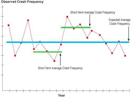
Regardless of the problem identification method used to identify locations or road segments with potential for improvement, an appropriate time period needs to be defined for the analysis.  As discussed, crash experience can vary at a location from year to year, so it is important that more than one year of data is used for the analysis.

Typically a minimum of three years of crash data is used for analysis.  Multiple years of data are preferable to avoid the regression to the mean phenomenon.  However, the use of multiple years of data can be misguided because the facility itself may have changed (e.g., adding a lane), the travel volume may have increased, or some other change has taken place that skews the analysis.  In addition, it is sometimes difficult to obtain adequate multiple years of data; therefore, it is often necessary to use a method for enhancing the estimate for sites with few years of data.  The problem can be addressed by supplementing the estimation for a site with the mean (and standard deviation) for comparable sites using safety performance functions and empirical bayes.

Regression to the Mean

When identifying potential safety issues, the analyst must be aware of the statistical phenomenon of regression to the mean (RTM).  RTM describes a situation in which crash rates are artificially high during the before period and would have been reduced even without an improvement to the site.  Programs focused on high-hazard locations, such as the HSIP, are vulnerable to the RTM bias which is perhaps the most important cause of erroneous conclusions in highway-related evaluations.  This threat is greatest when sites are chosen because of their extreme value (e.g., high number of crashes or crash rate) in a given time period.

When selecting high-hazard locations; the locations chosen are often those with the worst recent crash record.  It is generally true that crash frequency or rate at a given location, all things remaining equal, will vary from year to year around a fairly consistent mean value.  The mean value represents a measure of safety at the location.  The variations are usually due to the normal randomness of crash occurrence.  Because of random variation, the extreme cases chosen in one period are very likely to experience lower crash frequencies in the next period, and vice versa.  Simply stated; the highest get lower and the lowest get higher.

The specific concern in road safety is that one should not select sites for treatment if there is a high count in only one year because the count will tend to “regress” back toward the mean in subsequent years.  Put more directly, what happens “before” is not a good indicator of what might happen “after” in this situation.

Figure 2.2 shows an example to demonstrate this concept.  It shows the history of crashes at an intersection, which might have been identified as a high-hazard location in 2003 based upon the rise in crashes in 2002.

Figure 2.2 Data Series for Example Intersection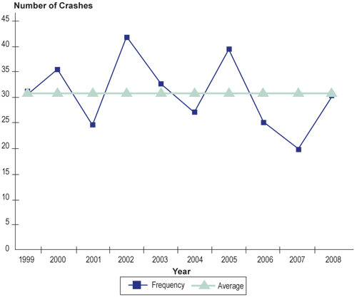

Even though a treatment may have been introduced early in 2003, any difference between the frequencies of crashes in 2002 and those in 2003 and 2004 (see Figure 2.3 would, to some unknown degree, not be attributed to the treatment, but to the RTM phenomenon.  The RTM phenomenon may cause the perceived effectiveness of a treatment to be overestimated.  Thus, there would be a “threat to validity” of any conclusions drawn from a simple comparison of conditions before and after a change at a site.

Figure 2.3 Example of Regression to the Mean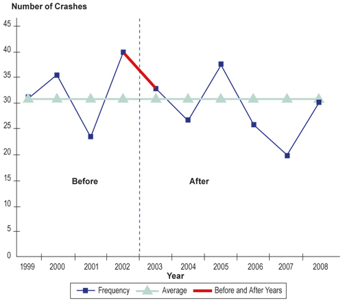

In fact, if a decision is made to forgo safety improvements at the site (e.g., due to lack of funds), the site would still be likely to show a reduction in crashes due to the natural variation in crash frequency.  However, one would not be inclined to conclude doing nothing is beneficial where a safety problem truly exists.

Safety Performance Functions

Safety performance functions (SPFs) are frequently used in the network screening and evaluation processes and can be used to reduce the effects of RTM.  They can be used to estimate the expected safety of a roadway segment or location based on similar facilities.

SPFs represent the change in mean crash frequency as ADT (or other exposure measure) increases or decreases.  The sites contained in an SPF are called comparable sites, because they are sites that are generally comparable to the site of interest.

SPFs are constructed using crash and exposure data from multiple comparable sites.  SPFs are constructed by plotting the crash and exposure data and then fitting a curve through the data using a negative binomial regression formula.  The resulting curve (or equation) is the SPF.

Numerous studies have been conducted to estimate SPFs for different types of facilities.  These SPFs have been compiled into safety analysis tools, such as SafetyAnalyst and the Highway Safety Manual (HSM).  However, since crash patterns may vary in different geographical areas, SPFs must be calibrated to reflect local conditions (e.g., driver population, climate, crash reporting thresholds, etc.).  Different entities have SPFs with different curves and use differing measures to represent exposure (e.g., annual average daily traffic, total entering vehicles, etc.).

Figure 2.4 depicts a typical SPF and shows crashes per mile per year for three data points (using triangles, squares, and diamonds as icons).  The small icons represent values for individual years while the large comparable icon represents the mean for several years.  Only three “sites” are shown in the figure, but a typical SPF may have from 100 to thousands of sites involved in its estimation.  One of the advantages of displaying data in this way is to show sites that exceed the mean crash frequency for comparable sites at the same level of exposure (AADT in this case).  One can think about sites with mean risk above the SPF as those with higher than average risk and those below the line as those with lower than average risk.

Figure 2.4 SPF with Individual Site Data

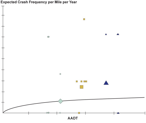
Note that the large triangle and large square lie above the SPF indicating mean expected crash frequency in excess of the average for comparable sites.  The large diamond lies directly on the SPF so for this site the expected crash frequency is virtually the same as the comparable sites.

Empirical Bayes

The Empirical Bayes (EB) method is a statistical method that combines the observed crash frequency with the predicted crash frequency using the SPF to calculate the expected crash frequency for a site of interest.  The EB method pulls the crash count towards the mean, accounting for the RTM bias.

The EB method is illustrated in Figure 2.5, which illustrates how the observed crash frequency is combined with the predicted crash frequency based on the SPF.  The EB method is applied to calculate an expected crash frequency or corrected value, which lies somewhere between the observed value and the predicted value from the SPF.  The EB method is discussed in more detail in Section 6.1.

Figure 2.5 Empirical Bayes Method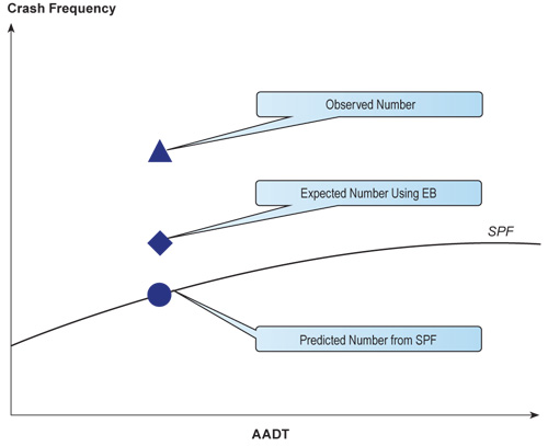

Defining a Site

Sites identified for safety improvements are either intersections or segments of roads; however, there is no clear definition of what length of a road segment should be considered as a site.  Typically roadways are sectioned off into segments of a fixed length, which varies from agency to agency.  The segment length used to identify potential sites for safety improvement is left to the agency’s discretion and does not need to be consistent for the entire data set, as long as the analysis accounts for segment length.  Many states are now implementing systemic improvements, which identify sites based on roadway characteristics, rather than individual sites.

2.4 Network Screening Process

Network screening is conducted to identify key crash types to address with systemic improvements or to identify specific sites with potential for safety improvement. 
The process will vary depending on whether the network screening is being conducted to identify systemic improvements or to identify sites with potential for improvement.

Identifying Safety Issues to Address with Systemic Safety Improvements

Analysis now focuses more on road segments, corridors, and even entire networks.  Analysts look beyond a particular location and concentrate on surrounding road segments for more efficient and effective countermeasure implementation.  Some states are implementing systemic improvements using countermeasures known to be effective.

A systemic highway safety improvement is a particular countermeasure, or set of countermeasures, implemented on all roadways or roadway sections where a crash type is linked with a particular roadway or traffic element.  Locations for implementing improvements are NOT based on the number or rate of crashes at particular locations, but on an analysis of what roadways share the “dangerous” elements that may be mitigated by the improvement.

The process for identifying potential safety issues to address with systemic improvements should build on the analysis used to develop the emphasis areas in the state Strategic Highway Safety Plan (SHSP).  The actual identification process may vary among states but typically involves the following three steps:

1. First, identify key crash types to address (e.g., run-off-road, median crossover), which is similar to selecting emphasis areas in the SHSP.  Typically the key crash types are selected based on the number and severity of crashes.
2. Next, identify characteristics of the facilities on which key crash types occur (e.g., rural versus urban, two-lane versus four-lane, divided versus undivided, on curve versus on tangent, type of intersection control, etc.).
3. Finally, set thresholds that further define the “high-risk” facilities on which to implement the countermeasures (e.g., AADT greater than 20,000 vehicles per day, horizontal curves greater than 7 degrees, median widths less than 50 feet, etc.).

As an example, through data analysis one state has identified a significant number of severe run-off-the-road crashes occurring on their rural two-lane roadways with horizontal curves.  After further looking into the analysis, they discovered most of these crashes were occurring on horizontal curves greater than seven degrees.  Based on their findings, they decided to look into proven effective countermeasures on horizontal curves and to implement them on all two-lane rural roadways with horizontal curves greater than seven degrees.

States should use the SHSP to guide or influence systemic improvements in their HSIP project selection process.  The emphasis areas identified in the SHSP can help states identify systemic improvements to include in the HSIP project selection process and, in some cases, address safety problems before they occur.

Once the key crash types and key characteristics are identified, the next step is to identify the appropriate countermeasure(s) for systemic improvements.  This step will be discussed in Unit 3.

Identifying Sites with Potential for Safety Improvement

The network screening process for identifying sites with potential to benefit from a safety improvement involves a comprehensive review of a selected roadway network to identify locations with a potential safety problem.  This process is typically conducted in four steps:

1. Identify and group the network elements;
2. Select problem identification methodology;
3. Select screening method; and
4. Screen and evaluate results.

The remainder of this section provides more detail on each of the four steps in the site identification process.

Identify and Group the Network Elements

The first step is to identify the network elements to be screened and group them into reference populations.  Elements that might be considered for the screening process include:  intersections, segments, facilities, ramps, ramp terminals, or at‑grade crossings which are then grouped by reference population or sites with similar characteristics.

By establishing a reference population, the performance at a particular site is compared to the expected safety of the reference population, yielding a relative measure of comparison for determining sites with potential for improvement.  Reference populations can be established based on several characteristics.

Intersections potentially may be grouped into reference populations based on:

• Traffic control (signalized, two-way or all-way stop control, yield control, roundabout);
• Number of approaches (three-leg, four-leg intersection);
• Cross-section (number of through and turning lanes);
• Functional classification (arterial, collector, local);
• Area type (urban, suburban, rural);
• Traffic volumes (million entering vehicles (MEV), peak hour volumes, or average daily traffic; including pedestrian, bicycle, trucks, bus volumes);
• Terrain (flat, rolling, or mountainous); and
• Turning movements.

Similarly, roadway segments may be grouped into reference populations based on:

• Area type (urban, suburban, rural);
• Number of lanes per direction;
• Functional classification (arterial, collector, local);
• Area type (urban, suburban, rural);
• Access density (driveway or intersection spacing);
• Traffic volumes (peak hour traffic, average annual daily traffic (AADT); including pedestrian, bicycle, trucks, bus volumes);
• Median type and/or width of median;
• Operating or posted speed; and
• Terrain (flat, rolling, or mountainous).

Intersections and roadways may be grouped based on multiple reference populations, which will depend on the available data.  For example, intersections might be grouped as urban signalized intersections of two arterials or urban signalized intersections of an arterial with a collector roadway.  Once the network elements have been grouped by reference populations, problem identification methods are selected to use in the evaluation.

Select Problem Identification Methodology

Selecting a problem identification methodology to use for the analysis of the network elements is the second step in the network screening process.  The evaluation can be based on one or multiple problem identification methods.  The use of multiple problem identification methods may provide more certainty in the evaluation, if the same sites are ranked among the top sites with multiple methods.

Several problem identification methodologies can be used to identify sites for safety improvements, and the specific problem identification method used varies from agency to agency.  Agencies should use problem identification methods in the network screening process that suit their specific purpose and available data.

The following are the 13 problem identification methods (Referred to as performance measures in the HSM.) identified in the Highway Safety Manual (HSM); however, states are using additional methods not included in the HSM:

1. Average Crash Frequency – Sites are ranked based on the total number of crashes or by a particular crash severity or type during a given time period.  The site with the highest number of crashes is ranked first.
2. Crash Rate – The crash rate normalizes the crash frequency based on exposure.
   Equivalent Property Damage Only (EPDO) Average Crash Frequency – Each crash is weighted based on the crash severity and the equivalent property damage only crash cost.
3. Relative Severity Index – Average monetary crash costs are assigned to each crash at a site, and the total average crash cost for a site is compared to the average crash cost for the reference population.
4. Critical Crash Rate – A critical crash rate or threshold value is calculated for each site and compared to the observed crash rate.  Sites with an observed crash rate greater than their critical crash rate are flagged for further investigation.
5. Excess Predicted Average Crash Frequency Using Method of Moments – With this method, the observed crash frequency for a site is adjusted based on the variance in the crash data and the average crash counts for a site’s reference population, which is then compared to the average frequency of crashes for the reference population.
6. Level of Service of Safety (LOSS) – This method compares the observed crash frequency and/or severity to the mean value predicted for the reference population using a SPF.  The difference between the two values yields a performance measure that ranges between LOSS I and LOSS IV, with LOSS I indicating a low potential for crash reduction and LOSS IV indicating a high potential for crash reduction.
7. Excess Predicted Average Crash Frequency Using SPFs – This method represents the difference between the observed crash frequency for the site and the predicted crash frequency based on the SPF with information specific to the site.
8. Probability of Specific Crash Types Exceeding Threshold Proportion – This method is based on the probability that the long-term proportion of a specific crash type exceeds a threshold proportion for the site’s reference population.
9. Excess Proportion of Specific Crash Types – This is the difference between the observed proportion of a specific crash type for a site and the threshold proportion for the reference population.
10. Expected Average Crash Frequency with EB Adjustment – The expected crash frequency is calculated using a calibrated SPF, which is then weighted with the observed crash frequency using the EB method.  The EB method accounts for regression to the mean bias and is discussed in detail in Unit 6.
11. EPDO Average Crash Frequency with EB Adjustment – This method combines the expected crash frequency method with EB adjustments and the EPDO crash frequency method.  The expected crash frequency is calculated using a calibrated SPF and weighted with the observed crash frequency using EB, which is then weighted based on crash severity and the equivalent property damage only cost.
12. Excess Expected Average Crash Frequency with EB Adjustment – The expected crash frequency determined from a SPF is weighted with the observed crash frequency using the EB method.  The resulting weighted crash frequency is then compared to the expected crash frequency using the SPF to determine the difference between the two values.

Each of these problem identification methodologies has different data needs, strengths, and weaknesses.  Table 2.1 summarizes the data needs, strengths, and weaknesses of the 13 problem identification methods.

Once the problem identification method(s) has been chosen for the evaluation, the next step is to select the screening method.

Table 2.1 Summary of Problem Identification Methodologies

Problem Identification Method	Data Inputs and Needs	Strengths	Weaknesses
Average Crash Frequency	Crashes by type and/or severity and location.	Simple; and May be applied to crashes by type and severity.	Does not account for RTM bias; Does not account for exposure; May overlook low-volume sites and overemphasize high-volume sites; and Does not identify a performance threshold.
Crash Rate	Crash counts and location; and Average Daily Traffic Volumes (ADT), Total Entering Volume (TEV), or Annual Average Daily Traffic Volumes (AADT).	Simple; and Can modify to account for severity if EPDO or RSI‑based crash count is used.	Does not account for RTM bias; Does not identify a performance threshold; May overemphasize sites with low volumes; and Comparisons cannot be made across sites with significantly different volumes.
Equivalent Property Damage Only (EPDO) Average Crash Frequency	Crashes by severity and location; and Fatal, injury, and PDO crash weighting factors.	Simple; and Considers crash severity.	Does not account for RTM bias; May overemphasize locations with a small number of severe crashes; Does not identify a performance threshold; and Does not account for traffic volume.
Relative Severity Index (RSI)	Crashes by type and location; and Crash costs by type.	Simple; and Considers crash type and crash severity.	Does not account for RTM bias; May overemphasize locations with small number of severe crashes; and Does not account for traffic volumes.
Critical Crash Rate	Crash counts and location; and Annual Average Daily Traffic Volumes (AADT).	Reduces exaggerated effect of sites with low volumes; Considers variance in crash data; Establishes a threshold for comparison; and Can be applied to specific crash type or severity.	Does not account for RTM bias.
Excess Predicted Average Crash Frequency Using Method of Moments	Crashes by type and location; and Traffic volume (AADT or ADT).	Establishes a threshold of expected performance for a site; Considers variance in crash data; and Allows sites of all types to be ranked in one list.	Does not account for RTM bias; Does not account for traffic volumes; and Ranking results are influenced by reference populations.
Level of Service of Safety	A minimum of three years crash data; Crashes by location; and SPF, overdispersion parameter, and all variable required for SPF.	Considers variance in crash data; Accounts for volume; and Establishes a threshold for comparison.	Effects of RTM bias may still be present.
Excess Predicted Average Crash Frequency Using SPFs	A minimum of three years crash data; Crashes by type, severity, and location; and Calibrated SPF.	Accounts for volume; and Establishes a threshold for comparison.	Requires calibrated SPF; and Effects of RTM may still be present in the results.
Probability of Specific Crash Types Exceeding Threshold Proportion	Crashes by type, severity, and location.	Also can be used as a diagnostic tool; Not affected by RTM bias; and Considers variance in crash data.	Does not account for traffic volumes; and Some sites may be identified for unusually low numbers of nontarget crash types.
Excess Proportion of Specific Crash Types	Crashes by type, severity, and location.	Also can be used as a diagnostic tool; Not affected by RTM bias; and Considers variance in crash data.	Does not account for traffic volumes; and Some sites may be identified for unusually low numbers of nontarget crash types.
Expected Average Crash Frequency with EB Adjustment	A minimum of three years crash data; Crashes by type, severity, and location; and Calibrated SPFs and overdispersion parameters.	Accounts for RTM.	Requires locally calibrated SPF; Requires rigorous analysis; and Data intensive.
EPDO Average Crash Frequency with EB Adjustment	A minimum of three years crash data; Crashes by type, severity, and location; Calibrated SPFs and overdispersion parameter; and Fatal, injury, and PDO crash weighting factors.	Accounts for RTM; and Considers crash severity.	May overemphasize locations with a small number of severe crashes depending on weighting factors used. Requires rigorous analysis; and Data intensive.
Excess Expected Average Crash Frequency with EB Adjustment	A minimum of three years crash data; Crashes by type, severity, and location; and Calibrated SPF and overdispersion parameter.	Accounts for RTM; and Establishes a threshold for comparison.	Requires locally calibrated SPF; Requires rigorous analysis; and Data intensive.

Source:    Highway Safety Manual, First Edition, Draft 3.1, April 2009.

Select Screening Method

Three screening methods can be used in the third step of the network screening process, including simple ranking, sliding window, or peak searching.  The method chosen is dependent on the reference population and the selected problem identification methodology.  Table 2.2 provides a summary of when each method is applicable.

Table 2.2 Screening Method Applications

Problem Identification Method	Segments			Nodes	Facilities
	Simple Ranking	Sliding Window	Peak Searching	Simple Ranking	Simple Ranking
Average Crash Frequency	Yes	Yes	No	Yes	Yes
Crash Rate	Yes	Yes	No	Yes	Yes
Equivalent Property Damage Only (EPDO) Average Crash Frequency	Yes	Yes	No	Yes	Yes
Relative Severity Index (RSI)	Yes	Yes	No	Yes	No
Critical Crash Rate	Yes	Yes	No	Yes	Yes
Excess Predicted Average Crash Frequency Using Method of Moments	Yes	Yes	No	Yes	No
Level of Service of Safety	Yes	Yes	No	Yes	No
Excess Predicted Average Crash Frequency Using SPFs	Yes	Yes	No	Yes	No
Probability of Specific Crash Types Exceeding Threshold Proportion	Yes	Yes	No	Yes	No
Excess Proportion of Specific Crash Types	Yes	Yes	No	Yes	No
Expected Average Crash Frequency with EB Adjustment	Yes	Yes	Yes	Yes	No
EPDO Average Crash Frequency with EB Adjustment	Yes	Yes	Yes	Yes	No
Excess Expected Average Crash Frequency with EB Adjustment	Yes	Yes	Yes	Yes	No

Source:   Highway Safety Manual, First Edition, Draft 3.1, April 2009.

Simple Ranking

As the name suggests, simple ranking is the simplest of the three screening methods and may be applicable for roadway segments, nodes (intersections, at‑grade rail crossings), or facilities.  The sites are ranked based on the highest potential for safety improvement or the greatest value of the selected problem identification methodology.  Sites with the highest calculated value are identified for further study.

The sliding window and peak-searching methods are only applicable for segment-based screening.  Segment-based screening identifies locations within a roadway segment that show the most potential for safety improvement on a study road segment, not including intersections.

Sliding Window

With the sliding window method, the value of the problem identification methodology selected is calculated for a specified segment length (e.g., 0.3 miles), and the segment is moved by a specified incremental distance (e.g., 0.1 miles) and calculated for the next segment across the entire segment.  The window that demonstrates the most potential for safety improvement out of the entire roadway segment is identified based on the maximum value.  When the window approaches a roadway segment boundary in the sliding window method, the segment length remains the same and the incremental distance is adjusted.  If the study roadway segment is less than the specified segment length, the window length equals the entire segment length.

Peak Searching

Similar to the sliding window method, the peak-searching method subdivides the individual roadway segments into windows of similar length; however, the peak-searching method is slightly more meticulous.  The roadway is first subdivided into 0.1-mile windows; with the exception of the last window which may overlap with the previous window.  The windows should not overlap.  The problem identification method is applied to each window and the resulting value is subject to a desired level of precision, which is based on the coefficient of variation of the value calculated using the problem identification method.  If none of the 0.1-mile segments meet the desired level of precision, the segment window is increased to 0.2 miles, and the process is repeated until a desired precision is reached or the window equals the entire segment length.  For example, if the desired level of precision is 0.2, and the calculated coefficient of variation for each segment is greater than 0.2, then none of the segments meet the screening criterion, and the segment length should be increased.

Screen and Evaluate Results

Finally, the selected problem identification method(s) and screening method(s) are applied to the study network.  The result will be a list of sites identified with potential for safety improvement with the sites most likely to benefit at the top of the list.  These sites should be studied further to determine the most effective countermeasures (discussed in Unit 3).

As mentioned previously, applying multiple problem identification methods to the same data set can improve the certainty of the site identification process.  Sites listed at the top of the list based on multiple problem identification methods should be investigated further.  To provide a better understanding of the network screening process, two example applications are provided.

Network Screening Applications for Identifying Sites

This section provides two example applications of the network screening process for identifying sites with potential for safety improvement using the EPDO average crash frequency and the excess predicted average crash frequency using SPFs.  The EPDO average crash frequency is included because it is a method currently used by many states in their screening process, and the excess predicted average crash frequency using SPFs was included because more states are starting to utilize SPFs in their screening process.  The HSM will provide greater detail and several examples of all the problem identification and screening methods.
For the sample applications, it is assumed that the network elements have been identified and grouped into reference populations.  All numbers used in the following examples are fictitious and provided for illustrative purposes only.  We begin with an explanation of how to apply the EPDO crash frequency to screen and evaluate the network.

Equivalent Property Damage Only (EPDO) Average Crash Frequency

The EPDO average crash frequency identifies sites with potential for safety improvement for all reference populations.  This method weights the frequency of crashes by severity to develop a score for each site.  The weighting factors are calculated based on the crash cost by severity relative to the cost of a property damage only crash.  The crash costs should include both direct (e.g., EMS, property damage, insurance, etc.) and indirect (e.g., pain and suffering, loss of life).  This method provides a ranking of sites based on the severity of the crashes.

1. The first step is to calculate the weighting factors for fatal, injury, and PDO crash severities using local data (if local data sources are not available, references have been provided in Section 4.3).  In some cases, fatal and injury crashes may be combined to avoid overemphasizing fatal crashes.  The weighting factors are calculated as follows:

2.   The weighting factors are applied to the sites based on the most severe injury for each crash to develop a score:

Where:

KF,i = crash frequency of fatal crashes on segment i;

KI,i = crash frequency of injury crashes on segment i; and

KPDO,i = crash frequency of PDO crashes on segment i.

3.  The sites are then ranked from highest to lowest.

Example

The following is a short example applying the EPDO average crash frequency to a roadway segment using the sliding window method.  The study roadway already is divided into segments of equal length.  The average crash costs and segment crash information is as follows:

• Average fatal crash cost = $6,800,000;
• Average injury crash cost = $390,000; and
• Average PDO crash cost = $12,000.

Not Applicable	Crash Count
Segment	Fatal	Injury	PDO
1a	0	22	8
1b	1	8	3
1c	0	16	5
1d	1	14	2
1e	0	19	6
1f	0	20	3

1. The first step is to calculate the weighting factors based on the given crash cost:

2.   Now the weighting factors are applied to each segment.  For Segment 1a:

The scores for the remaining segments are shown below.

Segment	Fatal		Injury		PDO		EPDO Score	Total Crashes
	Crash Count	Weighted Value	Crash Count	Weighted Value	Crash Count	Weighted Value
1a	0	0	22	715	8	8	723	30
1b	1	567	8	260	3	3	830	12
1c	0	0	16	520	5	5	525	21
1d	1	567	14	455	2	2	1,024	17
1e	0	0	19	618	6	6	624	25
1f	0	0	20	650	3	3	653	23

3.   For this study roadway, Segment 1d is ranked first.

Alternatively, a weighted average of the fatal and injury crashes could be used so that sites with fatal injuries are not overemphasized in the analysis.  If these crashes are weighted using the injury factor only, Segment 1a is ranked first as shown below.

Segment	Fatal and Injury		PDO		EPDO Score	Total Crashes
	Crash Count	Weighted Value	Crash Count	Weighted Value
1a	22	715	8	8	723	30
1b	9	293	3	3	296	12
1c	16	520	5	5	525	21
1d	15	488	2	2	490	17
1e	19	618	6	6	624	25
1f	20	650	3	3	653	23

It should be noted this method does not account for RTM or provide a threshold for comparing the crash experience with expected crash experience at similar sites.

Excess Predicted Average Crash Frequency Using SPFs

The excess predicted average crash frequency using SPFs is another problem identification method that can be used in the network screening process to compare a site’s observed crash frequency to the predicted crash frequency from a SPF.  The difference between the two values is the excess predicted average crash frequency.
It is once again assumed the focus has been established as identifying sites with potential for safety improvement and the network has been identified and grouped into reference populations.  In addition, it is assumed the appropriate calibrated SPFs have been obtained (SPFs can be obtained from the HSM and other research documents, but they should be calibrated to local conditions).

1. The first step is to tabulate the crashes by type, severity, and total each site for each reference population being screened:

   a. The crash counts are summarized as crashes per year at nodes; and

   b. The crashes are tabulated on a per mile per year basis for segments, either for the entire site or for the window of interest.

2. Use the appropriate SPF to calculate the estimated number of crashes (Ny), for each year (y), for the analysis period (y = 1, 2, …, Y).  For segments, the crashes should be expressed on a per mile basis (calculated for the entire site or the window of interest).  The number of estimated crashes for each year should then be summed together and divided by the number of years to summarize the crashes by year (or crashes per mile per year for segments).
   
   
3. The next step is to calculate the excess average crash frequency (Excess(K)) based on all the years of data:

Where:

Avg(Ki) = Average observed crash frequency for site (or window); and

Avg(N) = Average estimated crash frequency from SPF for site (or window).

  4.   The final step is to rank all of the sites in each reference population based on excess predicted average crash frequency.

Example

A numerical example is provided below using the excess predicted average crash frequency using SPFs as a problem identification method.  The given reference population is signalized four-legged intersections with the following three years of AADT and crash data.

Not Applicable	Year 1			Year 2			Year 3
	AADT		Total Observed Crashes	AADT		Total Observed Crashes	AADT		Total Observed Crashes
Intersection	Major Street	Minor Street		Major Street	Minor Street		Major Street	Minor Street
A	25,000	10,000	8	25,400	11,000	6	26,000	11,200	10
B	30,600	12,000	9	31,100	12,100	12	31,800	12,500	11
C	28,800	13,000	10	30,000	13,500	9	30,500	13,800	8
D	27,600	11,500	11	28,100	11,800	13	28,600	12,200	12

The calibrated SPF for signalized four-legged intersections in the area is:

Where:

NTOT = The SPF predicted number of total crashes;

AADTmaj = Average annual daily traffic on major roadway; and

AADTmin = Average annual daily traffic on minor roadway.

1. The first step is to total the crashes at each intersection during the study period and divide by the number of years.  For intersection A:

   Observed crashes per year = (8 + 6 + 10) crashes/3 years = 8 crashes per year

  2.   The SPF is used to calculate the estimated number of crashes for each year at each site. The estimated crashes for each year at a site are then added together and        divided by the number of years.  For intersection A:

Year 1:

Year 2:

Year 3:

Estimated crashes per year = (7.95 + 8.11 + 8.21) crashes/3 years = 8.09 crashes per year.

  3.   The excess is then calculated for each intersection.  For intersection A:

The first three steps are repeated for the remainder of the reference population, which is summarized in the following table.

Not Applicable	Year 1		Year 2		Year 3		Three-Year Total		Observed Crashes per Year	Predicted Crashes per Year	Excess Crash Frequency
Inter-section	Observed Crashes	Predicted Crashes with SPF	Observed Crashes	Predicted Crashes with SPF	Observed Crashes	Predicted Crashes with SPF	Observed Crashes	Predicted Crashes with SPF
A	8	7.95	6	8.11	10	8.21	24	24.26	8.00	8.09	-0.09
B	9	8.87	12	8.94	11	9.07	32	26.89	10.67	8.96	1.70
C	10	8.75	9	8.95	8	9.04	27	26.73	9.00	8.91	0.09
D	11	8.45	13	8.54	12	8.64	236	25.63	12.00	8.54	3.46

  4.   Finally the sites are ranked based on their excess predicted average crash frequency.

Intersection	Excess Crash Frequency
D	3.46
B	1.70
C	0.09
A	-0.09

Sites with an excess crash frequency greater than zero experience more crashes than expected, while sites with a value less than zero experience fewer crashes than expected.  Based on this method, intersection D has the greatest potential for safety improvement.

This section described the network screening process and many problem identification methodologies for use in identifying sites with potential for safety improvement, including example applications.  The HSM and SafetyAnalyst are tools that can assist the safety practitioner in identifying sites with improvement potential.

2.5 Summary

In this unit, we discussed the importance of quality data in safety planning and outlined resources and methods for improving data.  In addition, we addressed the network screening process for identifying potential safety issues to address with systemic improvements and for sites with potential for safety improvements.  Once the system problems or sites with potential for safety improvement have been identified, the next step is identifying contributing crash factors and countermeasures for addressing the problem – the focus of Unit 3.

< Previous

Table of Contents

Next >