U.S. Department of Transportation
Federal Highway Administration
1200 New Jersey Avenue, SE
Washington, DC 20590
202-366-4000
| < Previous | Table of Contents | Next > |
The ultimate measure of success for the HSIP is a reduction in motor vehicle related crashes and the resulting fatalities and serious injuries. SAFETEA‑LU established the HSIP as a core program and nearly doubled the funds for infrastructure safety. With the increased funding also came a required focus on results, which further heightensthe importance of the state’s procedures for evaluating individual projects and programs, as well as the overall HSIP program.
The goal of evaluation in the HSIP process is for agencies to estimate the effectiveness of highway safety improvements. The evaluation process reveals if the overall program has been successful in reaching performance goals established in the planning process, including its effectiveness in reducing the number of crashes, fatalities, and serious injuries or the potential for crashes. Evaluation results should flow back into the various HSIP components to improve future planning and implementation, ensure resources are used effectively, and increase the effectiveness of future safety improvements.
Unit 6 discusses project and program evaluations. It addresses CMFs, evaluation studies, program evaluation methods, and using evaluation feedback to impact future safety planning and decision-making. The unit does not detail statistical and economic assessment methodologies to determine the effectiveness of HSIP projects or programs in achieving their goals; these methodologies are addressed in the HSM.
Evaluation is critical to determine if a specific project or group of projects is achieving the desired results and to ensure the investments have been worthwhile. The evaluation will provide a quantitative estimate of the effects on safety of a specific countermeasure, project, or group of projects. The evaluation results can provide valuable information for future planning. For example, the evaluation of a particular countermeasure can be used to determine if it should be used at more sites.
The evaluation may include determining the effectiveness of:
The evaluation must be stated in terms related to the desired results. If the goal is to reduce the hazard to pedestrians at an intersection, at least one of the performance measures must gauge the affect on pedestrian-related crashes. Agencies should identify actionable and measurable performance goals (e.g., reduce the number of fatalities and serious injuries) for the evaluation.
A basic task of project evaluation is to measure conditions, including the performance measures, both before and after a change is made. The effectiveness of the change is determined by comparing change in the value of the performance measure (e.g., frequency or rate of crashes) with the change which would have been expected if the site had not been treated. This approach is appropriate whether one is evaluating the application of strategies at a site or subjects (e.g., drivers). The challenge is estimating the change in the performance measure without a treatment. It is especially difficult because all other things do not remain equal as noted earlier. Since crash rates can vary significantly from year to year, crash estimates are susceptible to regression to the mean (RTM).
In addition to project specific evaluations (single or multiple sites), agencies can use the results of evaluation studies to develop state-specific CMFs. By developing their own CMFs, states will have a more accurate indication of the countermeasure effects. Using a CMF developed by another agency does not necessarily account for actual driver, roadway, traffic, climate, or other characteristics in a state and may over or underestimate the effectiveness of a countermeasure. In addition, the methodology used by another agency to develop a CMF may be uncertain. Developing state-specific CMFs not only allows a state to evaluate the effectiveness of their efforts, it also verifies their efforts are working to improve safety.
As previously discussed in Unit 3, a CMF is the ratio of the expected number of crashes with a countermeasure to the expected number of crashes without a countermeasure.
![]()
Where:
CMF = CMF for treatment “t” implemented under conditions “a”;
Et = the expected crash frequency with the implemented treatment; and
Ea = the expected crash frequency under identical conditions but with no treatment.
When developing CMFs, it is not recommended to use data from only one site because it may overestimate the effectiveness of a change. It is best to use data from a minimum of 10 to 20 sites, as it is less biased and will produce a more reliable result.
Some states already develop their own CMFs based on past HSIP projects. Other states refine CMFs (or crash reduction factors) to account for local road conditions, crash severity, injury severity, collision manner, and weather condition. Lastly, other agencies use before/after EB analysis to revise CMFs, and use these factors to analyze and prioritize new programs and projects.
This section demonstrates the various evaluation methods that can be used to determine the effectiveness of a single project at a specific site or a group of similar projects, and also provides information related to calculating CMFs.
The three basic types of evaluations used to measure a safety improvement are:
Observational studies are more common in road safety evaluation because they consider safety improvements implemented to improve the road system, not improvements implemented solely to evaluate their effectiveness. Conversely, experimental studies evaluate safety improvements implemented for the purpose of measuring their effectiveness.
The remainder of the project evaluation section will outline these three evaluation methods.
Observational before/after studies are the most common approach used in safety effectiveness evaluation. An observational before/after study requires crash data and volume data from both before and after a safety improvement. These studies can be conducted for any site where improvements have been made; however, if a site was selected for an improvement because of an unusually high-crash frequency, evaluating this site may introduce the RTM bias.
Simple Before/After Evaluation
An observational before/after study conducted without consideration to nontreatment sites is referred to as a simple before/after evaluation. Figure 6.1 demonstrates a simple before/after evaluation.
In this figure and the series of figures that follows, the y‑axis represents the value of the performance measure (e.g., number of crashes, number of fatalities, etc.), and the x‑axis represents the time increment of the performance measure data (e.g., monthly, annually, etc.). The period between before and after measurements is shown by the vertical line, which can range from instantaneous (e.g., where the change may be a law coming into effect), to more than a year (e.g., where a period is required for construction and adjustment of traffic).
Figure 6.1 Simple Before/After Evaluation
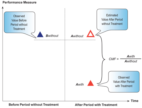
In a simple before/after evaluation, the average value of the performance measure for all treatment sites remains unchanged in the after period, as shown by the dashed line. The assumption is the expected value would remain the same as in the before period. This simplifying assumption weakens the ability to conclusively say the difference measured in the after period was due solely to the applied treatment. This approach is not recommended, and has sometimes been referred to as a naïve method.
As shown in Figure 6.1, a CMF can be developed using a simple before after study by taking the ratio of the observed value of the performance measure in the after period with the treatment to the estimated value of the performance measure in the after period without the treatment. However, this is not a preferred method for developing CMFs.
Observational before/after evaluations can incorporate nontreatment sites by using the EB method or by using a comparison group. These methods are preferred over a simple before/after evaluation.
Observational Before/After Evaluation Using Empirical Bayes Method
Incorporating the Empirical Bayes (EB) method into a before/after study compensates for the RTM bias. The EB method can be used to calculate a site’s expected crash frequency “E.” The EB analysis requires AADT and crash data for the treatment site for both before and after the treatment was implemented. The SPF, discussed in Unit 2, is incorporated into the EB analysis to determine the average crash frequency at similar sites. The sites expected crash frequency can be calculated is as follows:
![]()
Where:
![]()
μ = SP = The average number of crashes/(mile-year) on similar entities (determined from SPF);
Y = Number of years in evaluation period; and
![]() = Overdispersion parameter estimated per unit length for segments (calculated in the development of the SPF).
= Overdispersion parameter estimated per unit length for segments (calculated in the development of the SPF).
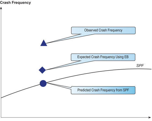
The EB method pulls the crash count towards the mean, accounting for RTM bias. Figure 6.2 illustrates how the observed crash frequency and the predicted crash frequency are combined to calculate a corrected value, which is the expected crash frequency using EB. The expected crash frequency will lie somewhere between the observed crash frequency and the predicted crash frequency from the SPF.
The reliability of the data affects the “weight.” The more reliable the data is, the more weight will go to the data; conversely, the less reliable the data is, the more the weight will go to the average.
The standard deviation of the estimated expected crash frequency can be calculated as follows:
![]()
Figure 6.2 Empirical Bayes Method
The following is an example application of the EB method to estimate the expected crash frequency (Hauer, 2001):
Given a 1.1-mile road segment with annual crash counts of 12, 7, and 8 over a three-year time period and an ADT of 4,000 vehicles per day (for all three years). The safety performance function for similar roads is 0.0224 x ADT0.564 crashes per mile-year with an overdispersion parameter ![]() = 3.25 per mile. The expected safety of the road is estimated as follows:
= 3.25 per mile. The expected safety of the road is estimated as follows:
![]()
3. Estimate the expected crash frequency:
![]()
E = 0.375 x 2.41 + (1-0.375) x (12 + 7 + 8) = 17.78 crashes in three years.
With a standard deviation:
![]() crashes in three years.
crashes in three years.
The expected number of crashes is 17.78 ± 3.35 crashes in three years or 5.39 ± 1.01 crashes/(mile-year).
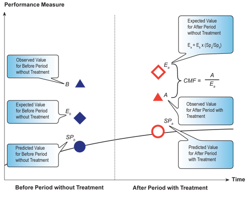
Figure 6.3 illustrates an observational before/after evaluation using the EB method. In the before period, the SPF is used to calculate the predicted value without the treatment, and then the observed value and the predicted value from the SPF are used to calculate an expected value. In the after period, the predicted value with the treatment is calculated using the SPF. The expected value in the after period without the treatment is then calculated by taking the ratio of the predicted values from the SPFs of the after “with” treatment to the before “without” treatment, and then multiplying this ratio by the expected value in the before period without the treatment. The expected value for the after period without the treatment can then be used to calculate a CMF by dividing the observed value in the after period with the treatment by this value.
Figure 6.3 Before/After Evaluation Using the EB Method
The EB method can be used by agencies to evaluate countermeasures and to calculate CMFs for specific sites as demonstrated in the following example.
Using the same 1.1-mile road segment from the previous example, a countermeasure was implemented to improve safety on the roadway. For the three years following the implementation of the countermeasure, the observed crash experience was 4, 7, and 5 crashes per year with an ADT of 4,200 for each year. The CMF for this project is calculated as follows:

Observational Before/After Evaluation Using a Comparison Group
Observational before/after studies can incorporate nontreatment sites into the evaluation by using a comparison group (or control sites). A comparison group typically consists of nontreated sites comparable in traffic volume, geometrics, and other site characteristics to the treated sites which do not have the improvement being evaluated. Crash and traffic volume data must be collected for the same time period for both the treated sites and the comparison group.
A valid comparison group is essential for conducting an observational before/after study using a comparison group. There should be consistency in the rate of change in crashes from year to year between the treatment sites and the comparison group, which is generally determined using a statistical test (refer to the HSM for detailed information on statistical tests).
The comparison group is used to estimate what would have happened if no treatment had been implemented. Figure 6.4 demonstrates the use of a comparison group.Figure 6.4 Before/After Evaluation Using a Comparison Group\
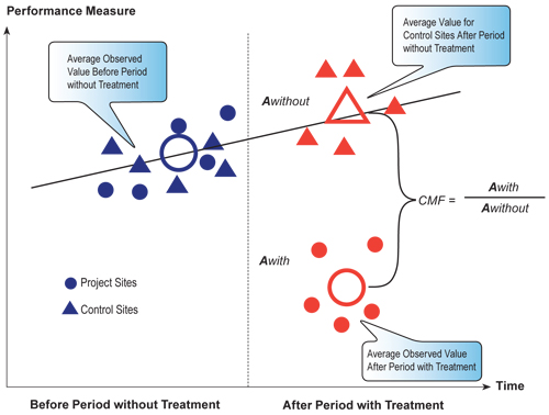
Similar to the previous figures, the period between before and after measurements is shown by the vertical line. With a comparison group, similar measurements are taken for both the comparison group and the sites being treated in both the before and after periods.
The values for the performance measure at the control sites are used to predict what would have happened if no change had occurred at a treatment sites. Figure 6.4 demonstrates how a change at the comparison sites could be estimated by using averages for the before and after period. It also shows individual site values may be used to perform a regression or trend analysis. Several statistical techniques are available to do this, some more “sophisticated” than others (the statistical techniques are described in the HSM). The choice of which technique to use is dependent upon the resources and time available to complete the evaluation, as well as the nature and significance of the treatment.
Figure 6.4 illustrates how a comparison group evaluation can be used to develop a CMF. The CMF is developed by dividing the average observed value of the performance measure for the project sites in the after period by the average observed value for the control sites in the after period.
In some cases, adequate comparison sites will not exist. An example would be what occurs as a result of a change in a state or Federal law intended to impact driving behavior (e.g., the national maximum speed limit, or lowering of the blood alcohol concentration (BAC) limit which defines DUI). In such cases, all sites or subjects which can be considered similar come under the category of “treated.” While not covered in this Manual, statistical procedures are available for conducting trend analyses which may be applied to this situation.
Observational Cross-Sectional Studies
In some cases, evaluations have been performed only after the fact, and data were not available for the performance measure during the before period. This might be necessary when:
Figure 6.5 Cross-Sectional Evaluation
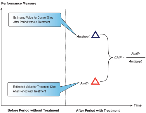
Figure 6.5 illustrates how a CMF is developed using an observational cross-sectional study. The CMF is the ratio of the estimated value of the performance measure for the treatment sites to the estimated value of the performance measure for the control sites.
Limitations exist when using a cross-sectional study. This approach limits the ability to be confident in the conclusions since trends over time are not taken into account. This method does not account for RTM, which threatens the validity of the results, especially if the treated sites were selected because they were identified as high-hazard locations. In addition, it is usually quite difficult to find control sites or subjects about which, or whom, it can be said there is true similarity, for the purposes of the evaluation.
Even in a well-designed evaluation, care should be taken to differentiate between the documented change and assumptions regarding the causes of the change. The stronger the evaluation, the more confident the evaluator can be that the strategies employed to improve safety brought about the change. However, limits to the confidence one can have exist, both of the type which can be measured statistically and due to the inability to account for the myriad of factors which may be present.
Experimental Before/After Studies
Experimental studies are those in which comparable sites with respect to traffic volumes and geometric features are randomly assigned to a treatment group or nontreatment group. In these studies, crash and traffic volume data is obtained for time periods before and after the treatment for the sites in the treatment group. Optionally, data also may be collected from sites in the nontreatment group during the same time period. One example of an experimental study is evaluation of the safety effectiveness of a new signing treatment.
The RTM bias is reduced in an experimental study compared to an observational study because of the random assignment of sites to the treatment or nontreatment groups. However, experimental studies are rarely used in highway safety due to the reluctance to randomly assign locations for improvements. This reluctance is largely due to budget and potential liability issues; however, a negative connotation may also be associated with denying improvements to certain populations or locations.
The necessary data will vary based on the evaluation method chosen. Table 6.1 summarizes the minimum data requirements for each study type.
Table 6.1 Safety Evaluation Method Data Requirements
Data Needs and Inputs |
Safety Evaluation Method |
|||
|---|---|---|---|---|
EB Before/After |
Before/After with Comparison Group |
Cross-Sectional Study |
Experimental Before/After |
|
10 to 20 treatment sites |
Yes |
Yes |
Yes |
Yes |
10 to 20 comparable |
Not Applicable |
Yes |
Yes |
Not Applicable |
3 to 5 years of crash and volume |
Yes |
Yes |
Not Applicable |
Yes |
3 to 5 years of crash and volume |
Yes |
Yes |
Yes |
Yes |
SPF for treatment site types |
Yes |
Yes |
Not Applicable |
|
SPF for nontreatment site types |
Not Applicable |
Yes |
Not Applicable |
|
Source: Highway Safety Manual, First Edition, Draft 3.1, April 2009.
Although a step-by-step process has not been provided for each of these methods, the HSM provides details on how to conduct each of these evaluations, and includes examples. Additional references on the techniques to use for highway safety evaluation and the EB method are included in the Resources section at the end of this document.
Agencies can use the safety effectiveness evaluations presented in this section to evaluate an individual project, group of projects, or a particular countermeasure. Cumulatively, the results of these evaluations feed into the assessment of the overall program.
Agencies conduct program-level evaluations to assess the HSIP’s contribution in reaching established performance goals. Section 1.7 addressed setting performance goals and more specific performance measures to determine the effectiveness of countermeasures and how changes in the system will affect performance. Now that the program has been implemented, it is time to analyze the data to determine the overall effectiveness of the HSIP and individual HSIP subprograms.
Agencies can utilize several different methods for assessing the overall success of their HSIP. States should perform evaluations that are most meaningful to them. Several common methods for measuring overall program success include, but are not limited to, process output and outcome performance measures, general statistics, trend analysis, benefit/cost analysis and safety culture. Each of these methods are described in more detail below.
One basic program evaluation method uses a compilation of output and outcome performance measures as a means to measure HSIP progress.
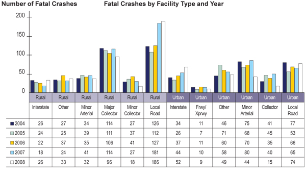
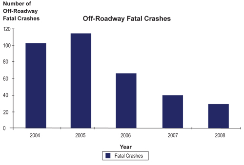
Agencies typically calculate crashes and crash rates (crashes per million vehicle-miles traveled) which are summarized by fatal crashes, injury crashes, property damage only crashes and total crashes. As an example, Figure 6.6 summarizes the annual fatal crashes by facility type. This summary is useful for determining if the program has been successful in reducing fatalities on particular roadway types.
Another method for measuring overall program success is to identify the crash trends for each of the agency’s focus areas. In this case, the established performance goal(s) are compared to the actual number of crashes for the past five-year period (although longer is preferred to better identify the trend). As an example, if one of the goals is to reduce the fatality rate by 50 percent by 2010, the trend rate can be determined by plotting the annual fatality rates as shown in Figure 6.7. The slope of the trend line identifies the average annual change in fatality rates.
Figure 6.7 Trend Analysis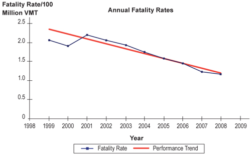
Trend lines help identify if the actual number of crashes each year is better or worse than would be expected if the trend stayed the same from year to year. In Figure 6.7, the end year data point is below the trend line, meaning the trend in fatality rates is better than would be expected had all other things been equal. Studying crash trends provides an indication of overall safety performance. However, since it is possible various programs or actions were causing this decline, additional evaluation of individual programs within the HSIP are beneficial for identifying which aspects of the program had the most impact on reducing fatalities.
Conducting a benefit/cost analysis of all HSIP-related projects provides another indicator of overall HSIP success. To conduct a benefit/cost analysis for the overall HSIP program, add the present value of the benefits for all HSIP projects together to get an overall benefit and add the present value of all of the project costs to get an overall cost. The benefit/cost ratio is calculated by dividing the present value of the overall program benefits by the present value of the overall program costs (Section 4.2 of this manual discusses benefit/cost analysis in detail). If the benefit/cost ratio is greater than one, the benefits of the program have outweighed the costs, and it provides some indication the program has shown success in improving safety. Typically, program benefit/cost analysis is conducted using three years data for both before and after implementation of improvements.
Qualitative measures also may demonstrate the effectiveness and success of the HSIP. For example, successful implementation of HSIP-related programs, strategies, and/or treatments may lead to policy or design standard changes. These policy and design standard changes result in safety treatments being applied across all projects and not just safety-specific projects. This reflects not only a policy-level change, but a shift in the safety culture of the agency.
States are expected to focus their HSIP resources on their areas of greatest need and those with the potential for the highest rate of return on the investment of HSIP funds. As the HSIP has evolved, one noteworthy change has been the shift in focus towards evaluation of individual HSIP programs. While it is beneficial to determine the overall effectiveness of a state’s HSIP in terms of achieving statewide performance goals; it is just as important to determine the success of specific HSIP-funded programs.
A highway safety program is a group of projects, not necessarily similar in type or location, implemented to achieve a common highway safety goal. Examples of highway safety programs include an established program administered by a Federal agency (e.g., Highway-Rail Grade Crossing Program), a systemic program to address a specific crash type (e.g., lane departures, “drift-off-the-roadway” crashes), and a speed management program combining engineering, enforcement, emergency response, and public education strategies designed to address a Strategic Highway Safety Plan (SHSP) emphasis area of speed-related crashes on selected rural road corridors.
Identifying programs that have the least amount of impact on the performance goals can result in subtle changes, such as new or additional treatments to move the program toward its intended purpose. Alternatively, implementation of successful programs and treatments implemented as part of the HSIP should continue.
Measures of program effectiveness include observed changes in the number, rate, and severity of traffic crashes resulting from the implementation of the program. Program effectiveness is also examined with respect to the benefits derived from the program given the cost of implementing the program.
The following examples of program evaluations provide an overview of how an agency might conduct an evaluation of each type of highway safety programs. Other examples of program evaluation criteria might better demonstrate the success of HSIP-related program.
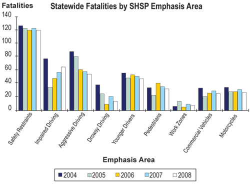
Similar to determining overall HSIP effectiveness, overall SHSP success can be seen in the crash trends for each of the emphasis area performance measures (i.e., fatalities and serious injuries, all crashes). Figure 6.8 illustrates a summary of statewide fatalities by SHSP emphasis area.
The evaluation process also must assess if the HSIP contributed to reaching the specific performance goals aligned with the state’s SHSP. Programs administered under the HSIP often target subsets of the SHSP emphasis areas or specific strategies (e.g., cable median barrier program or speed management program). States should evaluate the overall effectiveness of these programs.
As an example, if a state has been implementing a median guard cable program for the past several years, trends in cross median crashes should be evaluated. An effective approach is to compare the cross median fatalities to the miles of guard cable installed, as shown in Figure 6.9. This figure demonstrates a decrease in cross-median fatalities as the miles of median guard cable installation increased.
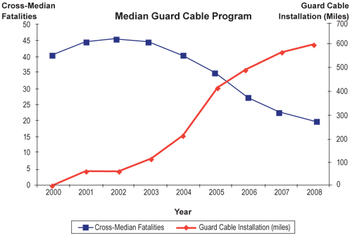
Source: Chandler (2007).
Figure 6.10 Systemic Treatment
The most common program evaluation challenges are related to data issues and available resources for conducting evaluations. Numerous reports indicate states are making progress in resolving data issues. Resolving resource issues associated with performing evaluations can include training, hiring additional staff, obtaining outside assistance, or identifying additional funding to support the oversight and conduct of the state’s evaluation efforts. Resolving data and resource issues will improve future HSIP planning and decision-making.
To identify some of these challenges, it is beneficial to periodically take a step back and conduct an assessment of the HSIP. An assessment allows states to review their HSIP, or elements of the program, to identify noteworthy practices and/or opportunities for improvement. The FHWA Office of Safety provides an HSIP Assessment Toolbox containing tools and resources to aid state DOTs in evaluating their HSIP program and processes. The toolbox provides information on several options available to conduct program assessments. The state can choose a self assessment, program review or peer exchange. States interested in obtaining more information about the HSIP Assessment Toolbox should contact their FHWA Division Office.
It is important to conduct evaluations to determine the overall effectiveness of the HSIP and of individual HSIP programs. However, evaluations can only provide benefit if they are used. The next section discusses the importance of using evaluation results to impact future actions.
Evaluation is a critical element in efforts to improve highway safety. Program and project evaluations help agencies determine which countermeasures are most effective in saving lives and reducing injuries. Agencies also may identify which countermeasures are not as effective as originally expected and decide not to use them in the future. The results of all evaluations should be captured in a knowledge base to improve future estimates of effectiveness and for consideration in future decision-making and planning.
As mentioned previously, states are conducting more rigorous statistical evaluations and refining CMFs based on crash data from past HSIP projects, using before/after EB analysis to revise CMFs, and using these findings to analyze and prioritize new programs and projects. At least one state has implemented a program which moves data from completed projects into a historical file that recalculates the CMFs.
Documentation is critical for the evaluation process. States should document key findings and issues occurring throughout the implementation process. Identifying potential issues and solutions before they occur can ease the implementation of similar programs and projects in the future.
To aid future planning, a state’s project analysis should:
Results of a well designed analysis can be fed back into making better estimates of effectiveness for use in planning future strategies.
Project results should be reported back to those who authorized them, and any stakeholders, as well as others in management involved in determining future projects. Decisions must be made on how to continue or expand the effort, if at all. If a program is to be continued or expanded, as in the case of a pilot study, the results of its assessment may suggest modifications. In some cases, a decision may be needed to remove what has been placed in the highway environment as part of the program, due to a negative impact. Even a “permanent” installation (e.g., rumble strips) requires a decision regarding investment for future maintenance, if its effectiveness is to continue.
Evaluation results also can provide justification for changing design standards and department policies. For example, countermeasures proven to be effective at improving safety based on the evaluation could be incorporated into new roadway design standards and included on all resurfacing projects.
One successful program evaluation strategy states employ is to monitoring performance in achieving fatality-reduction goals for specific SHSP emphasis areas and reporting those results periodically to state transportation leaders. By doing so, the evaluation process can lead to outcomes, such as further studies; the implementation of projects; refinement of planning, design, operational or maintenance standards; new practices and policies; and new regulations.
The HSIP development process is continuously evolving. States work to improve data deficiencies through their Traffic Records Coordinating Committee (TRCC), which in turn results in more accurate analysis for future programs. States make use of countermeasures proven effective based on project and program evaluations, and incorporate lessons learned into future HSIP and SHSP planning efforts. In combination, all these collaborative efforts result in moving the nation toward our goal of fewer motor vehicle-related fatal and serious injury crashes.
| < Previous | Table of Contents | Next > |

