U.S. Department of Transportation
Federal Highway Administration
1200 New Jersey Avenue, SE
Washington, DC 20590
202-366-4000
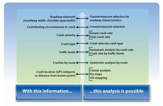
Collected data should be analyzed and reviewed to identify locations with safety issues or locations with potential for future safety issues, and to select countermeasures to improve safety. Depending on the completeness, accuracy, and timeliness of available data, a local jurisdiction can analyze that information in a number of ways. Figure 2 shows the relationship between data availability and the analysis potential for improved safety-related decision-making.
In Figure 2, as more types of data become available to the safety practitioner (moving up in the figure on the left), the ability to perform more in-depth safety analyses is enhanced (the list on the right of the figure). For example, if only the county and route of a crash location are known, analysis is limited to analyses by county and route. But as more specific location information is collected and stored, including milepost location or GPS coordinates, options like pin map cluster analysis and location comparisons become available. If additional exposure and roadway characteristic information can be linked to the location (traffic counts, roadway width, shoulder type) then even more robust analyses can be performed.
Figure 2. Relationship between Available Information and Analysis Possibilities
As noted, several types of data analysis can be conducted to support roadway safety depending on available crash, roadway and exposure data. They include:
Crash frequency is one of the simplest forms of crash data analysis. It is defined as the number of crashes occurring within a specific jurisdiction, on a roadway segment, or at an intersection. Multiple crashes occurring at the same location over a period of time may be an indication of a safety issue and should be investigated and addressed appropriately. This is referred to as "clustering". Crashes can be clustered by route, specific location on that route, or by intersection.
Example: County Road 220, in Potter's Grove, Rae County, is a 17-mile route that has 2,100 vehicles traveling on it each day. It had the following crash history over the past 5 years as shown in Table 2:
| Year | Crashes |
|---|---|
| 2005 | 2 |
| 2006 | 1 |
| 2007 | 6 |
| 2008 | 1 |
| 2009 | 2 |
| 5-year total | 12 |
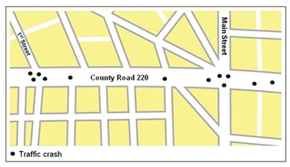
Beyond looking at the raw number of crashes on a route, a practitioner can plot the crash locations on a pin map to determine clustering, as shown in Figure 3. Data from this figure indicate that the CR220 & 1st Street and CR220 & Main Street intersections appear to have experienced multiple crashes over the 5-year study period.
Figure 3. Location of Crashes on County Road 220
Crashes are relatively rare events, so it is important that a safety analysis includes an adequate time frame of study. Crash averaging allows the practitioner to normalize crash data over a longer period than one year to account for annual anomalies that can skew analyses. Due to the randomness of traffic crashes, it is likely that any one year could have a much higher or lower number of crashes than the typical year. A rule of thumb is to collect data from the previous 3 to 5 years, with 3 years as a working minimum. A longer period of time increases the statistical value of the data; however, if the period is too long, there is a chance that the situation (e.g., roadway configuration, traffic volume and patterns) may have changed.
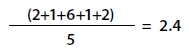
For County Road 220 (Table 2, above), the 5-year average of crashes is calculated by adding the total crashes from 2005-2009 and dividing by the period of 5 years:
Results show that County Road 220 averaged 2.4 crashes per year during that time period. Note that in 2007, the route experienced six crashes (five more than the year before and the year after), which might have caused the route to be "flagged" based on that single year of crashes. Averaging data across the 5-year analysis period provides a number more consistent with actual roadway conditions over time.
A Rolling Crash Average can also be used to achieve some normalcy from crash data. A Rolling Crash Average looks at the previous 3 to 5 years at more than one point in time. For example, the first data point could be 2001-2005 (a 5-year average). The next would be the 2002-2006 average, and so on. This technique further flattens the curve in an attempt to avoid inappropriate reaction to one or two statistically insignificant data points.
| Year | Crashes | 5-year period | Rolling Average |
|---|---|---|---|
| 2001 | 1 | ||
| 2002 | 3 | ||
| 2003 | 2 | ||
| 2004 | 0 | ||
| 2005 | 2 | 2001-2005 | 1.6 |
| 2006 | 1 | 2002-2006 | 1.6 |
| 2007 | 6 | 2003-2007 | 2.2 |
| 2008 | 1 | 2004-2008 | 2 |
| 2009 | 2 | 2005-2009 | 2.4 |
Table 3 shows that the rolling average of County Road 220 stayed relatively steady up to 2006, and then increased slightly from 2007 to 2009. A rolling average is commonly used to smooth out short-term fluctuations in the data and highlight longer-term trends. A study of the annual crashes shows one year with an atypically high number of crashes (six crashes in 2007). If crashes continue to hover near one or two crashes per year, the rolling average will quickly revert to that number as well.
The difference between looking at crashes per year and the rolling average, as shown in Table 3, is that the "peak" of the rolling average is only 2.4 versus six when looking at one year at a time. This supports a broader view of analysis by looking at the big picture and not focusing on a single data point.
A practitioner can also examine the trend of crashes over time to determine if crashes have been rising or falling. An increasing number of crashes may indicate an emerging safety issue. The crash history can be placed in a number of categories indicating both the number of crashes and the recent trend, such as:
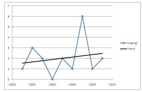
For County Road 220, Figure 4 provides a graphic representation of the crashes from 2001-2009 and the trend for these crashes. The figure indicates the crash number fluctuates from year to year and the trend is rising. The linear trend line can be calculated by a computer software program (e.g., Microsoft Excel) to provide a general idea of the rise or fall of traffic crashes based on the patterns of change from year to year. In this case, it would be worthwhile for the practitioner to perform two additional steps:
Figure 4. County Road 220 Crash Trends, 2001-2009
Crash rate analysis of the relative safety of a segment or intersection takes into account exposure data. The crash rate is calculated to determine relative safety compared to other similar roadways, segments, or intersections. Crash rate analysis typically uses exposure data in the form of traffic volumes or roadway mileage.
Typically, traffic volumes are expressed in the form of Annual Daily Traffic (ADT). As discussed above, traffic volume data is not always available at the local jurisdiction level. In these cases, rates can be calculated using other exposure data, such as roadway length. Information may be available from other agencies including county traffic or maintenance; the Metropolitan Planning Organization (MPO); the Regional Planning Organization (RPO); or from the State database.
The benefit of crash rate analysis is that it provides a more effective comparison of similar locations with safety issues. This allows for prioritization of these locations when considering safety improvements with limited resources.
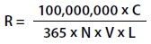
The crash rate for road segments is calculated as:
Where:
R = Crash rate for the road segment expressed as crashes per 100 million vehicle-miles of travel (VMT).
C = Total number of crashes in the study period.
N = Number of years of data.
V = Number of vehicles per day (both directions).9
L = Length of the roadway segment in miles.
If County Road 220 was being assessed with the following values:
C = 12 crashes over the past 5 years on this segment.
N = 5 years of data.
V = 2,100 vehicles per day.
L = 17 miles.
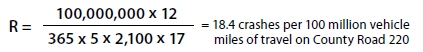
The resulting segment crash rate would be:
Depending on the details of crash reporting methods and crash history in a particular jurisdiction, a value of 18.4 may or may not be cause for additional study. The most appropriate use of this crash rate is to determine the relative safety of a roadway segment when compared to similar segment within a specific jurisdiction.
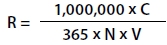
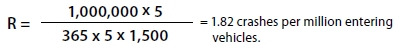
The most common equation used to calculate a crash rate at an intersection is as follows:
Where:
R = Crash rate for the intersection expressed as accidents per million entering vehicles (MEV).
C = Total number of intersection crashes in the study period.
N = Number of years of data.
V = Traffic volumes entering the intersection daily.10
If, for example, an intersection were being assessed with the following values:
C = 5 total crashes over the past 5 years.
N = 5 years of data.
V = 1,500 entering vehicles per day.
The resulting intersection crash rate would be:
Depending on the details of crash reporting methods and crash history in a particular jurisdiction, a value of 1.82 may or may not be cause for additional study. The most appropriate use of this crash rate is to determine the relative safety of an intersection when compared to similar intersections within a specific jurisdiction.
On many local roadways traffic volume information is not available. In these cases, other data can be used to make comparisons on a jurisdiction's system. As an example, route length can be used to develop a more accurate comparison of segment crashes than a simple crash frequency. Crashes per mile of roadway allow for an improved analysis across the system by improving the ability to compare crashes on roadways of differing lengths.
For example, two roadways could have the same number of crashes but different roadway lengths. In this case, traffic volume data is not available. By factoring in a measure of exposure (in this case route length), the calculation indicates that County Road 220 may be a more promising roadway for safety treatments.
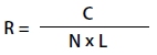
A "crashes per mile" rate for road segments is calculated as:
Where:
R = Crashes per mile for the road segment expressed as crashes per each 1 mile of roadway per year.
C = Total number of crashes in the study period.
N = Number of years of data.
L = Length of the roadway segment in miles.
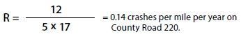
If County Road 220 was being assessed with the following values:
C = 12 crashes over the past 5 years on this segment.
N = 5 years of data.
L = 17 miles.
The resulting segment crash rate would be:
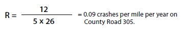
If Route B was being assessed with the following values:
C = 12 crashes over the past 5 years on this segment.
N = 5 years of data.
L = 26 miles.
The resulting segment crash rate would be:
The most appropriate use of any crash rate is as a relative value to compare the safety of a segment or intersection to similar locations in a specific jurisdiction. As shown in Table 4, the crash rate of County Road 220 is higher than County Road 305 due to its shorter route length.
| Roadway | Crashes (C) | Years of Data (N) | Length of segment (L) | Crashes per mile per year |
|---|---|---|---|---|
| County Road 220 | 12 | 5 | 17 miles | 0.14 |
| County Road 305 | 12 | 5 | 26 miles | 0.09 |
It is important to note that only roadways with similar cross-sections (e.g., two-lane, four-lane undivided, four-lane divided expressways) should be compared by section length.
Crash rates can be used to compare the crash experience of similar locations in the jurisdiction, region, and state.11 One method of comparing intersections or segments within a jurisdiction is to develop an average crash rate for the network. By calculating crash rates at a number of locations (intersections and segments) in the region, a baseline average for the comparison of future targeted locations can be developed. If resources are not available for this type of analysis, another source could be State highway agencies. State agencies typically develop average crash rates for different types of intersections and roadway segment cross-sections for statewide analyses.
Knowledge of the severity of crashes in a jurisdiction can assist practitioners in determining their safety needs. For example, the frequency of crashes at urban intersections may be higher than at rural curves, but in many cases the rural curve crashes are more severe. In addition, if two similar locations had the exact same number of crashes, it may be appropriate to select the location with more severe crashes to address first.
Local jurisdictions often do not have access to all the data desired for safety analysis. While much of the discussion focuses on examining a location's crash history, it is also important to identify locations on local rural roads that show potential for future crashes. Identifying these locations and proactively implementing safety improvements can potentially save lives.
Identifying and addressing locations with potential safety issues and no crash history can be accomplished in the following steps:
Federal and State studies have identified specific roadway features that can contribute to crashes. Additionally, these studies have identified tested and proven safety countermeasures to address these issues. Local practitioners should review available literature when considering these types of safety improvements on their network. See Appendix B for a list of resources.
Most States have developed data analysis tools that electronically analyze crash data and incorporate other types of data (e.g., roadway information, traffic volumes) to conduct comprehensive analyses. Often these tools are shared with local jurisdictions. For additional information, a local practitioner should contact the State highway agencies or State Local Technical Assistance Program (LTAP) center. Resources related to data analysis tools and methods currently in use are listed in Appendix B.
8 Data from this table will be used throughout this manual to illustrate different analysis methods. [ Return to note 8 ]
9 It is possible that traffic counts by direction are available from different years. In this case, a growth factor should be applied to the earlier data (based on historic trends at that site) so that it will be consistent with the newer information. [ Return to note 9 ]
10 It is possible that traffic counts on the roadways in this analysis are available from different years. In this case, a growth factor should be applied to the data (based on historic trends at that site) so that it will be consistent with the newest available counts. [ Return to note 10 ]
11 Similar is defined as similar in cross section, relatively similar traffic volumes (even if counts are unavailable), and roadway use (i.e., arterial, collector, local). [ Return to note 11 ]