U.S. Department of Transportation
Federal Highway Administration
1200 New Jersey Avenue, SE
Washington, DC 20590
202-366-4000
Safety assessment methods can be incorporated into all phases of the project development process. To demonstrate how an agency could continue to assess safety throughout the various project stages, the following urban street case study, referred to as a continuous case study, provides example problems that answer the following questions:
The detailed calculations for these questions are summarized in Sections 5.1, 5.2, and 5.3.
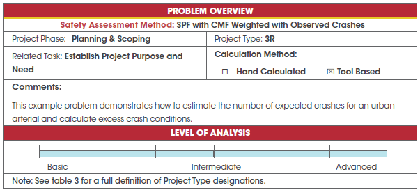
As part of planning and scoping activities, a transportation agency has identified an urban street targeted for renovation that experiences multiple-vehicle crashes involving vehicles turning left. The specific section of the urban street includes two segments and two signalized intersections. The street has a narrow divided median but does not have any left-turn lanes. The section is 1.85 miles in length and passes through a community that consists of commercial development near multiple-family residential dwellings, as shown on the aerial photo. The associated Project Type is a 3R project and the Related Task is to Establish Project Purpose and Need. How can the analyst estimate which, if any, of the road segments or intersections have more crashes than expected for a facility of this type?
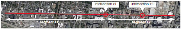
Source: ©Google Earth
Segment Data
The existing urban corridor has the following segment characteristics:
Characteristics unique to each segment are summarized in the following table:
| Roadway Segment Characteristic | Segment 1 | Segment 2 |
|---|---|---|
| Segment Length (miles) | 1.1 | 0.75 |
| Annual average daily traffic (vehicles per day) [3-year average value] | 13,300 | 11,500 |
| Commercial driveway count | 1 major, 17 minor | 3 major, 7 minor |
| Industrial/institutional driveway count | 2 major, 0 minor | 2 major, 0 minor |
| Residential driveway count | 1 major, 0 minor | 0 |
| Other driveway count | 0 | 0 |
Note: For the purposes of this example, a major driveway is assumed to have a minimum of 10 vehicles per hour during the peak periods.
| Crash Type/ Location | Observed Crash Frequency (crashes/yr) | 3-Year Average for Observed Crash Frequency (crashes/yr) | ||
|---|---|---|---|---|
| Year 1 | Year 2 | Year 3 | ||
| Multiple-vehicle non-driveway | ||||
| Segment 1 | 5 | 7 | 6 | 6 |
| Segment 2 | 2 | 1 | 3 | 2 |
| Single-vehicle | ||||
| Segment 1 | 3 | 3 | 3 | 3 |
| Segment 2 | 2 | 4 | 0 | 2 |
| Multiple-vehicle driveway-related | ||||
| Segment 1 | 1 | 3 | 2 | 2 |
| Segment 2 | 2 | 1 | 0 | 1 |
Intersection Data
The two public intersections located along the corridor have the following common characteristics:
Characteristics unique to each intersection are summarized in the following table:
| Signalized Intersection Characteristic | Intersection 1 | Intersection 2 |
|---|---|---|
| Major-road annual average daily traffic (vehicles per day) [3-year average value] | 13,300 | 11,500 |
| Minor-road annual average daily traffic (vehicles per day) [3-year average value] | 8,800 | 9,600 |
| Number of Bus Stops within 1,000 ft. of the Intersection | 11 | 7 |
| Schools within 1000 ft. of the Intersection | Present | Not present |
| Number of Alcohol Sales Establishments within 1,000 ft. of the Intersection | 0 | 1 |
Intersection crashes for the 3-year study period are shown as follows:
| Crash Type/Location | Observed Crash Frequency (crashes/yr) | 3-Year Average for Observed Crash Frequency (crashes/yr) | ||
|---|---|---|---|---|
| Year 1 | Year 2 | Year 3 | ||
| Multiple-vehicle non-driveway | ||||
| Intersection 1 | 3 | 2 | 4 | 3 |
| Intersection 2 | 2 | 2 | 2 | 2 |
| Single-vehicle | ||||
| Intersection 1 | 0 | 1 | 2 | 1 |
| Intersection 2 | 0 | 0 | 0 | 0 |
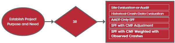
The analyst can first inspect Table 5 to identify potential safety assessment methods for a 3R project type and the Establish Project Purpose and Need task. Five potential methods may be considered for this analysis: two basic, two intermediate, and one advanced. Because the goal of this analysis is to assess whether the corridor experiences more crashes than would be expected for a facility of this type, a Site Evaluation or Audit would not provide this type of crash-specific information. The analyst plans to use the safety performance functions (SPF) from the Highway Safety Manual (HSM) for this assessment, so the AADT-Only SPF method can be removed from consideration. The Historical Crash Data Evaluation can be used to identify the type and location of crashes at the site, but does not provide information related to the number of crashes that could be expected at a similar facility and so this method is also removed from consideration. The two remaining methods can be used for the analysis.
The transportation agency noted the possibility that left-turn maneuvers may be an issue, and so the analyst selects the SPF with CMF Weighted with Observed Crashes option for this evaluation. This method enables subsequent evaluation of roadway characteristics, if needed, as the project development process progresses while also considering the crash history for the study corridor. The SPF with CMF Adjustment method, though not selected, is also a viable safety assessment method for this evaluation because it does allow the calculation of predicted crashes for similar facility types that could then be compared to the observed crashes.
The SPF with CMF Weighted with Observed Crashes method results in expected crash information and can be used for estimating the future performance of an existing facility or the future impact of minor geometric changes to an existing road (see Table 1). To most effectively use this approach, an agency should calibrate the SPF for its local jurisdiction. A calibration factor of 1.0 can be used if this information is not available, but the results will not be refined to local conditions. The results can, however, be used for comparative purposes.
After the expected number of crashes is calculated, a variety of analysis approaches can be used to then evaluate whether the corridor is overrepresented by crashes. For this assessment, the analyst will calculate the excess expected average crash frequency by comparing the number of expected crashes (unique to the study corridor) to the predicted number of crashes (representing roads with similar characteristics to the study corridor).
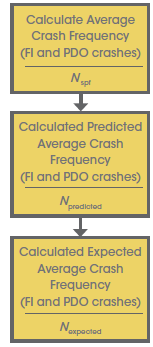
The HSM can be used to estimate the number of predicted crashes for an urban and suburban arterial by applying the procedures introduced in HSM Chapter 12 (pp. 12-1 to 12-122). By determining predicted crashes, the analyst can estimate how many crashes may be estimated for a specific road type with varying road conditions. Once the predicted number of crashes is known, the expected number of crashes for a specific site can be calculated by applying the Empirical Bayes Method summarized in HSM, Part C (Volume 2), pp. A-15 to A-23.
To further evaluate the calculated number of expected crashes, the analyst can then assess the various safety assessment performance measures summarized in Table 6 (based on HSM Table 4-1, p. 4-8). Because the selected Advanced safety assessment method (SPF with CMF Weighted with Observed Crashes) will result in the number of expected crashes, the analyst selects the excess expected crash frequency method to assess whether the crashes for the corridor exceed what can be typically estimated for a similar corridor. Additional information about this procedure is located in HSM Chapter 4 (p. 4-75 to 4-78).
The expected average crash frequency for the corridor segments and intersections can be calculated using the HSM "Smart Spreadsheets" available for download at: http://www. highwaysafetymanual.org/Pages/tools_sub.aspx#4. For this example problem, the analyst can use the "HSM prediction urban and rural arterials" spreadsheet tool.
STEP 1: Input the data for each segment and intersection into the spreadsheet tool.
The following graphic shows a representation of Worksheet 1A for Segment #1. This roadway segment worksheet includes input information similar to that shown in the HSM worksheet (see HSM p. 12-108). Segment #2 data is similarly input into a worksheet (not shown).
| General Information | Location Information | ||
|---|---|---|---|
| Analyst, Agency, or Company Date Performed: |
ABC DOT 06/15/16 | Roadway Roadway Section Jurisdication Analysis Year: |
Urban Corridor - Segment #1 MP 1.0 to MP 2.1 Small Town, USA 2015 |
| Input Data | Base Conditions | Site Conditions |
|---|---|---|
| Roadway type (2U, 3T, 4U, 4D, ST) | -- | 4D |
| Length of segment, L (mi) | -- | 1.1 |
| AADT (veh/day), AADTMAX=66,000 (veh/day) | -- | 13,300 |
| Type of on-street parking (none/parallel/angle) | None | Parallel (Comm/Ind) |
| Proportion of curb length with on-street parking | -- | 1 |
| Median width (ft) - for divided only | 15 | 10 |
| Lighting (present / not present) | Not Present | Present |
| Auto speed enforcement (present / not present) | Not Present | Not Present |
| Major commercial driveways (number) | -- | 1 |
| Minor commercial driveways (number) | -- | 17 |
| Major industrial / institutional driveways (number) | -- | 2 |
| Minor industrial / institutional driveways (number) | -- | 0 |
| Major residential driveways (number) | -- | 1 |
| Minor residential driveways (number) | -- | 0 |
| Other driveways (number) | -- | 0 |
| Speed Category | -- | Posted Speed Greater than 30 mph |
| Roadside fixed object density (fixed objects / mi) | 0 | 100 |
| Offset to roadside fixed objects (ft) [If greater than 30 or Not Present, input 30] | 30 | 10 |
| Calibration Factor, Cr | 1.00 | 1.00 |
Data for each of the study intersections can then be input into Worksheet 2A (see HSM p. 12-113). The following graphic depicts a representation of the Intersection #1 worksheet. Intersection #2 data is similarly included into a worksheet (not shown).
| General Information | Location Information | ||
|---|---|---|---|
| Analyst, Agency, or Company Date Performed: |
ABC DOT 06/15/16 | Roadway Roadway Section Jurisdication Analysis Year: |
Urban Corridor – Intersection #1 MP 1.0 to MP 2.1 Small Town, USA 2015 |
| Input Data | Base Conditions | Site Conditions |
|---|---|---|
| Intersection type (3ST, 3SG, 4ST, 4SG) | -- | 4SG |
| AADTMAJOR (veh/day), AADTMAX=67,700 (veh/day) | -- | 13,300 |
| AADTMINOR (veh/day), AADTMAX=33,400 (veh/day) | -- | 8,800 |
| Intersection lighting (present/not present) | Not Present | Present |
| Calibration factor, Ci | 1.00 | 1.00 |
| Data for unsignalized intersections only: | - | - |
| Number of major-road approaches with left-turn lanes (0,1,2) | 0 | 0 |
| Number of major-road approaches with right-turn lanes (0,1,2) | 0 | 0 |
| Data for signalized intersections only: | - | - |
| Number of approaches with left-turn lanes (0,1,2,3,4) [for 3SG, use maximum value of 3] | 0 | 0 |
| Number of approaches with right-turn lanes (0,1,2,3,4) [for 3SG, use maximum value of 3] | 0 | 0 |
| Number of approaches with left-turn signal phasing [for 3SG, use maximum value of 3] | -- | 0 |
| Type of left-turn signal phasing for Leg #1 | -- | Permissive |
| Type of left-turn signal phasing for Leg #2 | -- | Permissive |
| Type of left-turn signal phasing for Leg #3 | -- | Permissive |
| Type of left-turn signal phasing for Leg #4 (if applicable) | -- | Permissive |
| Number of approaches with right-turn-on-red prohibited [for 3SG, use maximum value of 3] | 0 | 0 |
| Intersection red light cameras (present/not present) | Not Present | Not Present |
| Sum of all pedestrian crossing volumes (PedVol) – Signalized intersections only | -- | 10 |
| Maximum number of lanes crossed by a pedestrian (nlanesx) | -- | 4 |
| Number of bus stops within 300 m (1,000 ft) of the intersection | 0 | 2 |
| Schools within 300 m (1,000 ft) of the intersection (present/not present) | Not Present | Present |
| Number of alcohol sales establishments within 300 m (1,000 ft) of the intersection | 0 | 0 |
STEP 2: Tabulate the predicted crash frequency for each segment and intersection.
The following graphics show representations of Worksheet 1L (see HSM p. 12-113) for Segment #1 and Worksheet 2L (see HSM p. 12-117) for Intersection #1. The analyst developed similar summaries (not shown) for Segment #2 and Intersection #2.
| Crash Severity Level | Predicted Average Crash Frequency Npredicted rs (crashes/year) (Total) from Worksheet 1K |
Roadway Segment Length (mi) | Crash Rate (crashes/mi/ year) (2)/(3) |
|---|---|---|---|
| Total | 5.8 | 1.10 | 5.3 |
| Fatal and Injury (FI) | 1.6 | 1.10 | 1.5 |
| Property Damage Only (PDO) | 4.2 | 1.10 | 3.8 |
| Crash Severity Level | Predicted Average Crash Frequency Npredicted int (crashes/year) (Total) from Worksheet 2K |
|---|---|
| Total | 3.6 |
| Fatal and Injury (FI) | 1.2 |
| Property Damage Only (PDO) | 2.4 |
STEP 3: Calculate the expected number of crashes for each segment and intersection.
The "Urban Site Total" worksheet tab in the spreadsheet can be used to summarize the predicted and observed crashes, apply the weighted adjustment factor, and calculate the expected average crash frequency. The summary results are depicted in the following representations for Worksheet 3A (see HSM p. 12-118). The bolded values represent the historical crash data.
| (1) Collision Type/Site Type | Predicted Average Crash Frequency | (5) Observed Crashes Npredicted (crashes/year) | Overdispersion Parameter, k | Weighted Adjustment, w (Equation A-5 from Part C Appendix) |
Expected Average Crash Frequency (Equation A-4 from Part C Appendix) |
||
|---|---|---|---|---|---|---|---|
(2) Npredicted (TOTAL) |
(3) Npredicted (FI) |
(4)Npredicted (PDO) |
|||||
| ROADWAY SEGMENTS – Multiple-vehicle non-driveway | |||||||
| Segment 1 | 3.931 | 1.137 | 2.795 | 6 | 1.32 | 0.162 | 5.666 |
| Segment 2 | 2.199 | 0.643 | 1.557 | 2 | 1.32 | 0.256 | 2.051 |
| ROADWAY SEGMENTS - Single-vehicle | |||||||
| Segment 1 | 1.231 | 0.194 | 1.037 | 3 | 0.86 | 0.486 | 2.141 |
| Segment 2 | 0.784 | 0.12 | 0.664 | 2 | 0.86 | 0.597 | 1.274 |
| ROADWAY SEGMENTS – Multiple-vehicle driveway-related | |||||||
| Segment 1 | 0.546 | 0.155 | 0.391 | 2 | 1.39 | 0.568 | 1.174 |
| Segment 2 | 0.372 | 0.106 | 0.266 | 1 | 1.39 | 0.659 | 0.586 |
| INTERSECTIONS – Multiple-vehicle | |||||||
| Intersection 1 | 3.208 | 1.007 | 2.201 | 3 | 0.39 | 0.444 | 3.092 |
| Intersection 2 | 2.801 | 0.864 | 1.937 | 2 | 0.39 | 0.478 | 2.383 |
| INTERSECTIONS - Single-vehicle | |||||||
| Intersection 1 | 0.248 | 0.073 | 0.175 | 1 | 0.36 | 0.918 | 0.31 |
| Intersection 2 | 0.23 | 0.071 | 0.159 | 0 | 0.36 | 0.924 | 0.212 |
| COMBINED (sum of column) | 15.551 | 4.369 | 11.182 | 22 | -- | -- | 18.889 |
STEP 4: Calculate the excess crashes by segment or intersection.
Based on the weighting of the observed and predicted crashes in Step 3, the analyst can calculate the excess expected average crash frequency to identify corridor segments or intersections with more than the expected number of crashes. Computing this measure requires the tabulation of the following quantities:
The excess value is calculated by subtracting the predicted average crash frequency from the expected average crash frequency. The following table summarizes the total crash statistics using this approach.
| Crash Type / Site Type | Predicted Average Crash Frequency (crashes/yr) | Expected Average Crash Frequency (crashes/yr) | Excess Calculated as Expected minus Predicted (crashes/yr) |
|---|---|---|---|
| Multiple-vehicle non-driveway | |||
| Segment 1 | 3.9 | 5.7 | 1.8 |
| Segment 2 | 2.2 | 2.1 | -0.1 |
| Single-vehicle | |||
| Segment 1 | 1.2 | 2.1 | 0.9 |
| Segment 2 | 0.8 | 1.3 | 0.5 |
| Multiple-vehicle driveway-related | |||
| Segment 1 | 0.6 | 1.2 | 0.6 |
| Segment 2 | 0.4 | 0.6 | 0.2 |
| Multiple-vehicle | |||
| Intersection 1 | 3.2 | 3.1 | -0.1 |
| Intersection 2 | 2.8 | 2.4 | -0.4 |
| Single-vehicle | |||
| Intersection 1 | 0.2 | 0.3 | 0.1 |
| Intersection 2 | 0.2 | 0.2 | 0 |
| Corridor Total | 15.6 | 18.9 | 3.3 |
Based on the excess expected average crash frequencies calculated in Step 4, the largest excess of crashes is found to occur on Segment 1. The overall street section is found to experience 3 to 4 more crashes per year than would be predicted for a similar facility.
The study location does not have left-turn lanes present but does include a 10-ft. median. This physical constraint requires the analyst to assume a segment roadway type that is a four-lane divided arterial (4D). Similarly, the parallel parking along the entire corridor length requires a value of 1 for the proportion of curb length with on-street parking. Because the curb length does not extend into the intersections, the total corridor length should not be used for determining this proportion value.
During the selection of the appropriate safety assessment method, the analyst also identified the SPF with CMF Adjustment as a candidate assessment method to consider. Because this method is classified as an Intermediate safety assessment method, the procedure results in predicted crashes for a facility type. The use of this alternative analysis method would require a safety assessment performance measure (see Table 6) other than the excess expected average crash value. The companion performance measure procedure to use with predicted crashes that will address the analyst's question of over-represented locations is the Excess Predicted Average Crash Frequency using SPFs noted in the performance measures table.
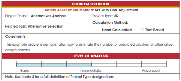
The analyst next conducted the alternative evaluations task for the improvement project for the four-lane divided urban arterial corridor identified in Section 5.1. After determining that the corridor does experience a higher-than-expected crash frequency, the analyst examined the crash predictions more closely to evaluate low-cost redesign options that could be implemented within the current right-of-way limits. The initial study identified Segment #1 as the section of road with the greatest number of expected crashes compared to predicted crashes, so the analyst is focused on alternatives that can be applied to that 1-mile segment.
The alternatives currently under consideration include:
The Project Type is 3R and the Related Task is Alternative Selection. How can the analyst compare the estimated crash frequency for the existing configuration to Option #1, Option #2, and Option #3?
The site data is the same as that presented in the Section 5.1 data summary. The modifications are expected to occur in 2 years, and at that time the AADT value is projected to increase moderately from the current 13,300 vpd value to 13,725 vpd.
The analyst can first review the potential safety assessment methods shown in Table 8. The Alternative Selection task and the 3R project type are associated with five safety assessment methods: two basic, two intermediate, and one advanced. For this evaluation, the analyst intends to compare the number of estimated crashes for three low-cost options and contrast these values to the number of crashes for the current segment. Since a CMF-based method enables the specific consideration of a change in road characteristics, the safety assessment methods that use CMFs are applicable for this analysis. Traffic volume information is also available, so a safety assessment method that is volume-based can be used. Based on these considerations, the AADT-Only SPF method, which does not directly capture changes in road characteristics, can be eliminated from further consideration. The analyst would like to incorporate both the calculations conducted for the initial assessment as well as the moderate increase in traffic volume. Consequently, the analyst eliminates the methods that do not use an SPF (i.e., CMF Applied to Observed Crashes and CMF Relative Comparison).
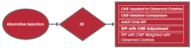
The two remaining safety assessment methods include SPF with CMF Adjustment and SPF with CMF Weighted with Observed Crashes. The analyst may elect to use one or both of these methods. Because the modifications can be expected to change the future number of crashes at the site, the analyst selects the SPF with CMF Adjustment method so that weighting with observed crashes for a modified roadway does not introduce unexpected biases. The SPF with CMF Weighted with Observed Crashes method can be used to evaluate the future impact of minor geometric changes to an existing road (per Table 1), but since the threshold of "minor geometric changes" can vary, the analyst elects not to use this particular method.
Ultimately, the analyst selects the SPF with CMF Adjustment method for the assessment. To use this analysis method most effectively, an agency should calibrate the SPF for its local jurisdiction. A calibration factor of 1.0 can be used if this information is not available, but the results will not be refined to location conditions. For the purposes of this assessment, the SPF method can be used for comparison.
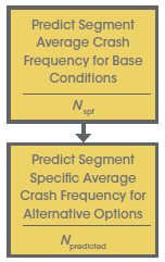
The HSM can be used to estimate the number of predicted crashes for an urban and suburban arterial by applying the procedures introduced in HSM Chapter 12 (pp. 12-1 to 12-122). By determining predicted crashes, the analyst can estimate how many crashes may be associated with a specific road type with varying road conditions. Once the predicted number of crashes is known, the analyst can compare the estimated safety performance of the varying options to identify optimal designs.
The predicted average crash frequency for the corridor segments and intersections can be calculated using the HSM "Smart Spreadsheets" available for download at: http://www.highwaysafetymanual.org/Pages/tools_sub.aspx#4. For this example problem, the analyst can use the "HSM prediction urban and rural arterials" spreadsheet tool.
STEP 1: Input the data for the study segment (referred to as Segment #1 in Section 5) into the spreadsheet tool.
This evaluation should use the future AADT value of 13,725 vpd. The following graphic shows a representation of Worksheet 1A for Segment #1, Option #3. This roadway segment worksheet includes input information similar to that shown in the HSM worksheet (see HSM p. 12-108). Information for existing Segment #1 conditions, Option 1, and Option 2 are similarly input into a worksheet (not shown).
| General Information | Location Information | ||
|---|---|---|---|
| Analyst, Agency, or Company Date Performed: |
ABC DOT 06/15/16 | Roadway Roadway Section Jurisdication Analysis Year: |
Urban Corridor-Segment #1 MP 1.0 to MP 2.1 Small Town, USA 2015 |
| Input Data | Base Conditions | Site Conditions |
|---|---|---|
| Intersection type (2U, 3T, 4U, 4D, ST) | -- | 4D |
| Length of segment, L (mi) | -- | 1.0 |
| AADT (veh/day), AADTMAX=66,000 (veh/day) | -- | 13,725 |
| Type of on-street parking (none/parallel/angle) | None | Parallel (Comm/Ind) |
| Proportion of curb length with on-street parking | -- | 0.5 |
| Median width (ft) - for divided only | 15 | 210 |
| Lighting (present / not present) | Not present | Present |
| Auto speed enforcement (present / not present) | Not present | Present |
| Major commercial driveways (number) | -- | 1 |
| Minor commercial driveways (number) | -- | 17 |
| Major industrial / institutional driveways (number) | -- | 2 |
| Minor industrial / institutional driveways (number) | -- | 0 |
| Major residential driveways (number) | -- | 1 |
| Minor residential driveways (number) | -- | 0 |
| Other driveways (number) | -- | 0 |
| Speed Category | -- | Posted Speed Greater than 30 mph |
| Roadside fixed object density (fixed objects / mi) | 0 | 50 |
| Offset to roadside fixed objects (ft) [If greater than 30 or Not Present, input 30] | 30 | 10 |
| Calibration Factor, Cr | 1.00 | 1.00 |
STEP 2: Calculate the number of predicted crashes for the study year.
At the completion of Step 1, the spreadsheet tools automatically calculated the predicted number of crashes for the existing conditions and for the three candidate options. To review example results for the intersection calculations, see the summary results of the predicted crashes for Option 3 (shown in Worksheet 1L). The analyst calculated similar summary results (not shown) for the Existing configuration, Option 1, and Option 2 (using the AADT value of 13,725 vpd as previously noted).
| Crash Severity Level | Predicted Average Crash Frequency Npredicted rs (crashes/year) (Total) from Worksheet 1K |
Roadway Segment Length (mi) | Crash Rate (crashes/mi/ year) (2)/(3) |
|---|---|---|---|
| Total | 4.2 | 1.10 | 3.8 |
| Fatal and Injury (FI) | 1.2 | 1.10 | 1.1 |
| Property Damage Only (PDO) | 3.0 | 1.10 | 2.8 |
Step 3: Summarize Findings.
The analyst's ultimate goal is to assess how much the three options have the potential to reduce the number of crashes predicted for the study segment 2 years into the future (when the AADT is 13,725 vpd). In addition to the total number of predicted crashes, the crash severity information is important to note. The following table summarizes these results.
| Roadway Improvement Scenario | Predicted Number of FI Crashes (crashes/yr) | Potential Reduction in FI Crashes (crashes/yr) | Percent Reduction in FI Crashes | Predicted Number of Total Crashes (crashes/yr) | Potential Reduction in Total Crashes (crashes/yr) | Percent Reduction in Total Crashes |
|---|---|---|---|---|---|---|
| Existing Configuration | 1.7 | N/A | N/A | 6.1 | N/A | N/A |
| Option 1 – Reduce on-street parking by 50% | 1.3 | 1.7 – 1.3 = 0.4 | 23.50% | 4.8 | 6.1 – 4.8 = 1.3 | 21.30% |
| Option 2 – Reduce the number of roadside objects to 50 per mile | 1.5 | 1.7 – 1.5 = 0.2 | 11.80% | 5.3 | 6.1 – 5.3 = 0.8 | 13.10% |
| Option 3 – Reduce on-street parking by 50% and reduce the number of roadside objects to 50 per mile | 1.2 | 1.7 – 1.2 – 0.5 | 29.40% | 4.2 | 6.1 – 4.2 = 1.9 | 31.10% |
Note: N/A = not applicable.
Based solely on an evaluation of the predicted number of crashes, reducing the on-street parking to approximately 50 percent of the curb length (Option #1) results in a 21.3 percent total crash reduction. If the number of roadside objects is reduced to 50 per mile (from the current 100 per mile) and the road is not otherwise modified (Option #2), the reduction in total number of crashes can be estimated to be approximately 13.1 percent. For the alternative that reduces the on-street parking and the roadside object density (Option #3), the reduction in the total number of crashes can be similarly estimated as a 31.1 percent. The number of fatal and injury crashes for the existing roadway segment is equivalent to less than two per year. This value is based on SPFs that have not been calibrated to the region. For all three options, the reduction in the number of fatal and injury crashes is similar to the trend observed for total crashes with reductions of 23.5 percent , 11.8 percent, and 29.4 percent for Option 1, 2, and 3 respectively.
For the conditions outlined in this problem, the minor modifications to the corridor appear to result in modest crash reductions. The number of predicted crashes can be used as input into a cost benefit study to assess whether the investment is economically justified. The analyst should use caution when assessing the results of this analysis due to the small number of crashes (less than 10). These calculations are based only on predicted crash performance, but do not consider potential operational issues. For example, limiting the on-street parking can potentially provide additional operational benefits to the adjacent travel lane.
The HSM procedures require the analyst to understand how SPFs and CMFs equate to the base conditions associated with the procedure. Incorrect use of these values can introduce erroneous results. This example compared the crash predictions, so a calibration factor with a value of 1.0 can be used for comparison purposes. If the analyst would like to record findings as crash frequency instead of percent reduction in the number of crashes, calibrated SPFs with known calibration factors should be used for the analysis. A more detailed analysis during the design phase would provide additional useful information about predicted crashes.
A common method for evaluating design alternatives is to use CMF comparisons that do not directly consider traffic volume. This approach is less reliable than the predictive methods, but can be used to evaluate alternatives when an SPF is not available for the condition or when a simple comparison between two alternatives is all that is needed.
The analyst can also use the advanced safety assessment method to further evaluate existing conditions and future designs with minor changes. Future configurations that include major changes are not suitable for the SPF with CMF Weighted with Observed Crashes method as the observed crashes would no longer be representative of the new configuration.
This problem is based on the scenario for Segment #1 as shown in Section 5.2.
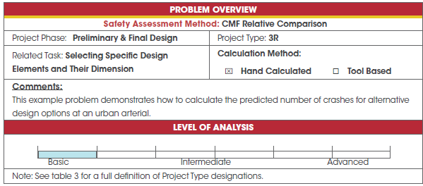
During the project development design phase, the transportation agency notified the analyst that on-street parking will be reduced by 50 percent for the entire corridor. This design change will result in complete removal of on-street parking at the intersection approaches for the corridor described in Section 5.1. The transportation agency intends to use the "recovered" space to make room for turn lanes at Intersection #1. The turn lanes will only be added on the primary corridor approaches (and not on the intersecting streets). The Project Type is 3R and the Related Task is Selecting Specific Design Elements and Their Dimensions. How can the analyst estimate the annual percentage reduction in crashes for installing a left-turn lane compared with the estimated reduction from installing a right-turn lane at Intersection #1?
The site data is the same as that presented in the Section 5.1 data summary. Right-turn-on-red will continue to be permitted on all approaches.
The analyst can first review the potential safety assessment methods shown in Table 9. The Selecting Specific Design Elements and Their Dimensions task and the 3R project type are associated with all seven candidate safety assessment methods. For this evaluation, the analyst intends to compare the estimated percent reduction in crashes for the two turn-lane options, so a CMF-based method that considers varying geometric characteristics is needed. As a result, the analyst may eliminate the Site Evaluation or Audit, the Historical Crash Data Evaluation, and the AADT-Only SPF safety assessment methods from further consideration. The addition of a turn lane at Intersection #1 is a minor geometric change, so any of the remaining four methods should be suitable for the turn lane analysis. Because all four of the CMF-based methods should provide similar results for this comparison, the analyst selects the basic method that does not require extensive data – CMF Relative Comparison. The analyst could also have used one of the remaining SPF-based methods with minimal additional effort as a continuation of the previous calculations conducted, as illustrated in Sections 5.1 and 5.2.
Chapter 12 (p. 12-24 to 12-26) and Chapter 14 (p. 14-23 to 14-26) of the HSM, as well as the FHWA-sponsored CMF Clearinghouse (www.cmfclearinghouse.org) collectively include a wide variety of CMFs for varying turn lane configurations. These CMF resources identify the base conditions and applicable site applications for the individual countermeasure of interest.
The CMF Relative Comparison safety assessment method can be used to compare potential countermeasures or treatments to identify the treatment most likely to have the greatest impact on reducing crashes. The only data requirement for this basic safety assessment method is the value for each CMF representing the candidate treatments for the same "before" characteristics and crash types.
To perform this assessment, the analyst reviews the CMF values for the two turn-lane options and compares their relative values. The information for the two CMFs is summarized in the following table. Recall that a CMF value less than 1.0 is associated with a larger reduction in future crashes when compared to a CMF with a value equal to 1.0 (assumed to have no real effect on reducing crashes). Based on this simple comparison, the analyst concludes that the recommended treatments, in order of priority, should be:
| Proposed Treatment | CMF (S.E.) | Crash Type (Base Condition) | Crash Severity | Source |
|---|---|---|---|---|
| Install left-turn lane on two signalized intersection approaches | 0.81 (0.13) | ★ ★ ★ All crash types and roadway types |
All | HSM Table 12-24, p. 12-43, HSM Table 14-12, p. 14-23, and CMF Clearinghouse at http://www.cmfclearinghouse.org/detail.cfm?facid=270#commentanchor |
| Install right-turn lane on two signalized intersection approaches | 0.92 (0.03) | ★ ★ ★ ★ ★ All crash types and rural road-way types |
All | HSM Table 12-26, p. 12-44, HSM Table 14-15, p. 14-26, and CMF Clearinghouse at http://www.cmfclearinghouse.org/detail.cfm?facid=290#commentanchor |
Note: ★ = CMF Clearinghouse Star Rating. CMF = crash modification factor. HSM = Highway Safety Manual. S.E. = standard error.
Based on the relative comparison of CMFs method, the analyst concluded that the addition of a left-turn lane on the two major approaches for Intersection #1 is a more effective option for reducing crashes than adding a right-turn lane. This assessment is based on the historic crash performance of left-turn and right-turn lanes and their associated CMFs and does not account for design features such as length of turn lane or operational features including consideration of turning volumes. A comprehensive assessment that addresses these issues should be performed as well during the design phase of the project development process.
A wide variety of CMF values are available for turn lanes. The selection of appropriate CMFs should include verification of appropriate base conditions, confirmation of consistent crash types between compared CMFs, and selection of higher quality CMFs based on small standard error values or higher star ratings (if using the CMF Clearinghouse). A common error associated with selection of CMFs is the selection of values that do not have applicable "before" conditions.
For this analysis, four candidate safety assessment methods emerged as viable options for the analysis. For the three methods that were not selected, the CMF value is multiplied by the observed or the predicted number of crashes. Though these techniques will result in numeric answers that generally represent the estimated reduction in crashes, they will all provide a similar answer to the analyst's question providing that the same CMF values are used for all of the evaluations. For this reason, any of the four CMF-based safety assessment methods is suitable for this analysis. The analyst selected the CMF Relative Comparison method based on the comparative nature of the question and recognized that, for this condition, this simple approach would provide similar findings as one of the more complex analysis methods and could be performed quickly with minimal data requirements.

