Scale and Scope of Safety Assessment Methods in the Project Development Process

Chapter 2. Planning and Scoping Applications

Planning and scoping activities occur early in the project development process and involve identifying the needs and range of actions, alternatives, and impacts to be addressed as part of the specific project scope. This Guide specifically focuses on project-level (rather than system-level) planning activities.

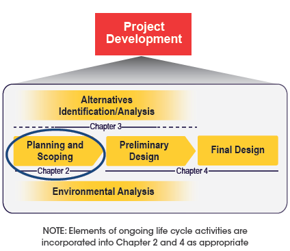
Figure 3. The Project Development Cycle and Corresponding
Planning and Scoping Chapter

Common considerations in this project development phase vary based on the type of project and may include operational efficiency, construction cost, right-of-way needs, effects on the human and natural environment, and safety.

This chapter provides information to help practitioners select safety assessment methods suitable for addressing questions about safety performance that arise during planning and scoping based upon the related task and project type. This Guide describes planning- and scoping-related tasks in three general categories:

• Conduct preliminary planning and needs assessment,
• Establish project purpose and need, and
• Establish project scope.

Preliminary planning and needs assessment occurs early in project development and may be part of a corridor or project planning study. The goal of this task is to assess the current and future needs of a transportation facility. As the planning process evolves, the transportation agency will establish a project purpose and need where the term "purpose" can generally be defined as what will be addressed and the "need" provides data to support that purpose. Following some level of project planning, the transportation agency can then establish the project scope, which often includes identifying and diagnosing opportunities to reduce crashes and then determining potential limits and types of treatments or mitigation strategies.

Table 5 identifies the safety assessment methods generally suitable for tasks related to planning and scoping and the objective of their safety performance analysis. The check marks in Table 5 suggest suitable safety assessment methods for each related task and objective and are, in some cases, distinguished by project type. In this context, the term "suitable" means that the method generally has the capability to address the safety performance related analysis objective with the data typically available for the related task and project type.

The following example questions demonstrate the type of questions the analyst may develop at the beginning of the safety assessment. These questions are based on the example problems included in this chapter.

1. How does the analyst assess where the limited funding could be most effectively spent?
2. What can the analyst do to assess if there is actually a need for safety treatments at this location?
3. How can the analyst estimate the safety performance of previously identified candidate low-cost countermeasures?
4. How can the analyst estimate which curves are functioning as anticipated and which ones could benefit from low-cost treatments?
5. How does the analyst estimate the reduction in the number of fatal and injury crashes due to these potential incremental improvements?

Table 5 shows that the level of predictive reliability generally increases along the spectrum of methods from basic to advanced. At the same time, the required resources for the analysis also will increase. In some cases, it may not be feasible to implement the preferred safety assessment method fully due to limitations in site information, crash data, traffic volume, or similar information. For example, the Basic safety assessment method for a CMF Applied to Observed Crashes cannot be executed if historic crash data is not available.

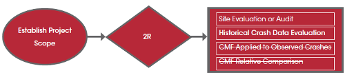
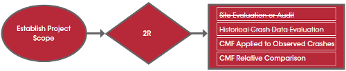
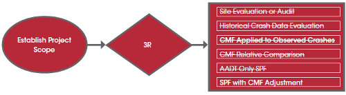
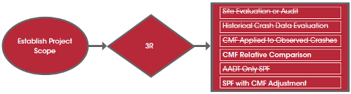
The approach for selecting a safety assessment method for planning and scoping looks like this:

Figure 4. The Approach for Selecting a Safety Assessment Method for
Planning and Scoping

A second safety assessment decision is the selection of the appropriate performance measure for the specific study question. In some cases, the performance measure may simply be based on average crash frequency or crash rate for an existing facility. Often, however, the performance measure is used to estimate some future performance (referred to as estimated, predicted, or expected crashes). Table 6 demonstrates several of these potential performance measures and their companion needs.

Related Task	Objective	Project Type	Basic				Intermediate		Advanced
			Observed Crashes			CMF Relative Comparison	Predicted Crashes		Expected Crashes
			Site Evaluation or Audit	Historical Crash Data Evaluation	CMF Applied to Observed Crashes		AADT-Only SPF	SPF with CMF Adjustment	SPF with CMF Weighted with Observed Crashes
Safety Assessments: (Increasing Level of Predictive Reliability from Left to Right)
Preliminary Planning and Needs Assessment	Characterize E5isting Safety Performance	All	✔6	✔6
Establish Project Purpose and Need	Diagnose Safety Issues the Project Should Address	2R	✔	✔
		3R, 4R	✔	✔			✔	✔9	✔10
		NL					✔	✔
Establish Project Scope	Refine Extent of Project and Safety Assessment Needs	2R	✔	✔5	✔7	✔7
		3R	✔	✔	✔	✔	✔	✔8
		4R	✔	✔	✔	✔	✔	✔	✔
		NL					✔	✔
Data Requirements: Increasing Level of Resources Needed)
Road Type1			✔		✔	✔	✔	✔	✔
Road Characteristics2			✔		✔	✔		✔	✔
Traffic Volume (vpd)3							✔	✔	✔
Observed Crash Data4			✔	✔	✔				✔

¹Road Type refers to rural two-lane highway, rural multi-lane highway, urban freeway, etc.
²Road Characteristics includes physical features such as lane widths, access density, etc.
₃Traffic Volume is the ADT or AADT in vehicles per day.
⁴Observed Crash Data represents the historic crash data at the study site for a period of more than 1 year (preferably 3 to 5 years).
⁵See Example Problem 2.1.
⁶See Example Problem 2.2.
⁷See Example Problem 2.3.
⁸See Example Problem 2.4.
⁹See Example Problem 2.5.
¹⁰See Example Problem 5.1.
Note: R2 = resurfacing existing facilities. R3 = major rehabilitation of an existing facility. R4 = major retrofit construction efforts. NL = highway construction at a new location. ✔ = suitable safety assessment method. ADT = average daily traffic. AADT = annual average daily traffic.

Table 6. Safety Assessment Performance Measures and Data Needs

Performance Measure	Data Requirements			Other Inputs
	Road Type / Characteristic	Traffic Volume	Observed Crash Data
Average Crash Frequency	✔		✔
Crash Rate	✔	✔	✔
Equivalent Property Damage Only (EPDO) Average Crash Frequency	✔		✔	EPDO Weighting Factors
Relative Severity Index	✔		✔	Relative Severity Indices
Critical Rate	✔	✔	✔
Excess Predicted Average Crash Frequency Using Method of Moments	✔	✔	✔
Level of Service of Safety	✔	✔	✔	Calibrated SPF with Overdispersion Parameter
Excess Predicted Average Crash Frequency Using SPFs	✔	✔	✔	Calibrated SPF
Probability of Specific Crash Types Exceeding Threshold Proportion	✔		✔
Excess Proportion of Specific Crash Types	✔		✔
Expected Average Crash Frequency with EB Adjustment	✔	✔	✔	Calibrated SPF with Overdispersion Parameter
EPDO Average Crash Frequency with EB Adjustment	✔	✔	✔	Calibrated SPF with Overdispersion Parameter & EPDO Weighting Factors
Excess Expected Average Crash Frequency with EB Adjustment	✔	✔	✔	Calibrated SPF with Overdispersion Parameter

Note: SPF = Safety Performance Function, EB = Empirical Bayes
Source: Adapted from the AASHTO Highway Safety Manual, Table 4-1, p. 4-8.

This chapter provides examples that demonstrate the selection process for the planning and scoping safety assessment methods. These examples are simplified hypothetical problems intended to illustrate the thought process for selecting a method and demonstrate how to apply the method to answer the associated safety question.

2.1 Priority Ranking Urban Signalized Intersections based on Pedestrian Crashes

Problem Overview

• Safety Assessment Method: Historical Crash Data Evaluation
• Project Phase: Planning & Scoping
• Project Type: 2R
• Related Task: Establish Project Scope
• Calculation Method: Hand Calculated
• Comments: This example problem demonstrates how to prioritize potential intersection improvements based on crash data.

Level of Analysis

Note: See table 3 for a full definition of Project Type designations.

Problem Description

As part of planning and scoping activities, a city has identified six candidate intersections for rehabilitation of pedestrian facilities; however, the city needs to narrow the list to only four of the sites. The associated Project Type is 2R and the Related Task is to Establish Project Scope. The expected improvements will include replacing/widening the sidewalks and installing/updating crosswalks. How does the analyst assess where the limited funding could be most effectively spent?

Summary of Available Data:

Table 7 presents a 3-year summary of observed crashes for the six signalized intersections. The sidewalks and crosswalks currently located at the intersections are of similar age and design. Pedestrian and vehicle volumes are unknown. Additional site information can be obtained, if needed, by reviewing aerial photographs or by visiting the six intersection locations.

Table 7. Example Summary of Available Data

Intersection Number	Number of Crashes (Three Years)		Number of Crashes (Average per Year)
	K+A* Pedestrian Crashes	Total Crashes	K+A* Pedestrian Crashes	Total Crashes
1	12	144	4	48
2	6	141	2	47
3	12	99	4	33
4	18	99	6	33
5	9	150	3	50
6	12	96	4	32
Average	11.5	121.5	3.8	40.5

*K+A refers to fatal and serious injury crashes.

Analysis

Selecting Appropriate Safety Assessment Method(s):

The analyst can first review the potential safety assessment methods shown in Table 5. The Establish Project Scope task and the 2R project type are associated with one of the four Basic safety assessment methods shown in Table 5. Table 1 (see Chapter 1) indicates that an evaluation of existing performance can be accomplished with the Site Evaluation or Audit or Historical Crash Data Evaluation safety assessment methods. The CMF-based methods require the use of CMF values as key elements of the analysis. Recall that a CMF commonly represents the change in the number of crashes due to varying a road characteristic. The analyst plans to use consistent improvements for the four selected intersections, and so the CMF assessment methods are not informative for this analysis.

The analyst can narrow down the prospective analysis approach to the remaining two basic safety assessment methods of Site Evaluation or Audit or Historical Crash Data Evaluation. A review of the data requirements for the safety assessment methods shown in Table 5 confirms that observed crash data is required or recommended for both assessment methods. In addition, the road type and road characteristics can be considered if a site evaluation is the selected assessment method. The requirements for each of the two assessments are comparable, and the analyst may choose to perform one or both.

Because every intersection is unique and site evaluations or audits can help isolate location-specific issues but may not help to establish priorities, the analyst selected the Historical Crash Data Evaluation method for the initial ranking of sites. The Site Evaluation or Audit method could then be conducted to reinforce the recommendations resulting from this Historical Crash Data Evaluation effort.

Linkage to the Highway Safety Manual (HSM):

The HSM provides a list of potential ranking methods commonly used for network screening purposes. These are summarized in Table 6 (based on HSM Table 4-1, p. 4-8). Several potential performance measures shown in Table 6 may be suitable for this screening, but may also require additional data not available for these sites. Two potentially suitable performance measures are (1) Average Crash Frequency (HSM p. 4-24), and (2) Excess Proportions of Specific Crash Types (HSM p. 4-52). In addition, the HSM includes suggestions for site evaluations if the analyst elects to pursue the additional Site Evaluation or Audit assessment method (HSM Chapter 5, pp. 5-1 to 5-24).

Detailed Analysis:

The average crash frequency can be ranked for K+A pedestrian crashes or for total crashes. Because the focus of this analysis is on improved pedestrian facilities and the expectation is to reduce the number of fatal or serious injury pedestrian crashes, evaluating K+A pedestrian crashes is important. In some locations, crash report information for this type of pedestrian crash may be limited. Similarly, a review of total crashes may help further clarify prevailing conditions at the intersection that are not clearly indicated when evaluating K+A pedestrian crashes alone. For these reasons, evaluation of these crashes can be complimented with a safety assessment of total crashes to confirm overall issues that may contribute to the number of crashes at the intersection.

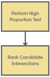
Where possible, the crash frequency method can be applied to locations with similar volumes. The excess proportions of specific crash types method ranks sites based on the proportion of a target crash type–in this case, K+A pedestrian crashes. The following steps summarize these calculations.

STEP 1: Summarize the crash data.

Develop a summary table that includes average K+A pedestrian crashes per year, average total intersection crashes per year, and associated K+A pedestrian proportion of total crashes. A threshold to assess the proportion of the K+A pedestrian crashes at each site would be the total proportion of all K+A pedestrian crashes for the six potential locations.

The threshold proportion is calculated as 23 ÷ 243 = 0.09. Locations with K+A pedestrian proportion of total crash values greater 0.09 merit consideration, based on this performance measure, during the ranking process.

Intersection Number	Average K+A Pedestrian Crashes per Year	Total Intersection Crashes per Year	K+A Pedestrian Proportion of Total Crashes1	Ranking by K+A Pedestrian Crash Frequency	Ranking by Total Crash Frequency	Ranking by Proportion
1	4	48	0.08	2	2	4
2	2	47	0.04	6	3	6
3	4	33	0.12	2	4	3
4	6	33	0.18	1	4	1
5	3	50	0.06	5	1	5
6	4	32	0.13	2	6	2
Total	23	243	N/A	N/A	N/A	N/A

¹ The proportion of total crashes is calculated by dividing K+A pedestrian crashes by total intersection crashes.
Note: N/A = Not applicable. The threshold proportion of K+A pedestrian crashes (for these 6 sites) is 0.09. Shaded cells represent the top ranked intersections for the specific performance measure.

STEP 2: Assess calculation of variance and probabilities.

The excess proportions ranking method calculations can be expanded to calculate the probability that the K+A pedestrian crashes exceed the threshold proportion. This process requires an additional calculation of a sample variance and the development of a probability to rank the sites that exceeded the threshold proportion. For this analysis, the analyst intends to select four intersections for improvement. Upon inspection, it is notable that only three of the intersections exceed the proportion and so all three will be considered. As a result, the analyst does not elect to compute the additional assessment values that are based on the simple variance.

STEP 3: Select and treat the highest ranked overrepresented sites.

Ranking based on the crash proportion test can be expected to produce different results than when the intersections are ranked by the average frequency of pedestrian crashes only or by total crashes. The shading in the summary table represents the top ranked intersections for each column. The four most critical intersections, based on the K+A Pedestrian Crash Frequency ranking, are Intersections #1, 3, 4, and 6. For intersections based solely on total crashes, Intersections #1, 2, and 5 are ranked the highest. Intersections #3 and 4 tied for fourth place. The ranking based on proportion includes sites where the proportion exceeds the overall threshold proportion value of 0.09 (or 9 percent) for all six intersections. This resulted in identification of Intersections #3, 4, and 6. Though the proportion value did not exceed 0.09, Intersection #1 did rank fourth using this proportion ranking method.

Intersections #1, 3, and 4 may be the clear priorities since they were ranked in the top four for all three ranking methods. The selection of the 4th priority among the remaining intersections boils down to a judgment call between intersections with more total crashes (#1 and 5) versus the intersection with more pedestrian K&A crashes (#6).

Findings

Interpreting the Results:

This simple analysis identified three intersections that have an overrepresented proportion of K+A pedestrian crashes. The intersection rankings based on total crashes provide very different recommendations than rankings based on average K+A pedestrian crashes or their associated proportion. Indications are that the analyst may want to recommend improving Intersections #1, 3, 4, and 6; however, the agency may want to evaluate additional site features (i.e. traffic volume, pedestrian crossing distance, etc.) to further confirm the sites with the greatest potential for K+A pedestrian crash reduction.

Possible Errors to Avoid:

Analysts should guard against making decisions about intersections involving a small number of crashes or using only 1 or 2 years of crash data. For the purposes of an intersection ranking analysis, a small number of crashes can be assumed to be less than 10 total crashes per year. Analysts should use a minimum of 3 years of crash data.

This demonstration included three common ranking methods. All three methods produce different results; therefore, using multiple ranking methods and selecting locations that are highly ranked by more than one ranking procedure will enable practitioners to consider varying dimensions of pedestrian and intersection safety.

Alternative Analysis Approaches:

The focus on evaluating observed K+A pedestrian crashes resulted in the analyst evaluating three performance measures associated with the Historical Crash Data Evaluation safety assessment method. If traffic volume information can be acquired, this analysis could be expanded to consider additional performance measures shown in Table 6, such as the crash rate or critical rate measures. As the project shifts from the planning to the design phase, the analyst will assemble more detailed site-specific information. At that time, additional analysis procedures that incorporate CMFs and/or SPFs can strengthen the overall analysis.

2.2 Conducting Site Evaluations Supplemented by Collision Diagrams for an Urban Arterial Intersection

Problem Overview

• Safety Assessment Method: Site Evaluation or Audit
• Project Phase: Planning & Scoping
• Project Type: 2R
• Related Task: Preliminary Planning & Needs Assessment
• Calculation Method: Hand Calculated
• Comments: This example problem demonstrates early project evaluation diagnostics for determining if a need exists.

Level of Analysis

Note: See table 3 for a full definition of Project Type designations.

Problem Description

The city has been asked to determine whether the entrance from an urban arterial to an unsignalized commercial driveway is in need of safety enhancements. In recent years, this location has experienced a number of minor crashes near the driveway entrance. The associated Project Type is 2R and the Related Task can be classified as Preliminary Planning and Needs Assessment. What can the analyst do to find out whether there is actually a need for safety treatments at this location?

Summary of Available Data:

The urban arterial corridor has two-way traffic with a total of six through lanes in the region of the unsignalized driveway, as shown on the following aerial photograph.

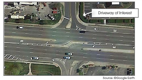
The annual average daily traffic (AADT) for the study corridor (at the driveway location) is 8,400 vpd. The 3-year crash information for this location includes three angle crashes and five rear end crashes for a 3-year total of eight crashes. This information is summarized in the following table.

Mile point	Time / date	Direction of Travel for V1, V2, V3	KABCO Severity Level	Maneuver Type	Light Condition	Road Surface Condition	Weather Condition
Angle Crashes:
19.16	18:18 / 1-17-13	North, West	C	V1: Turning Left, V2: Straight	Dusk	Dry	Clear / Cloudy
19.13	07:25 / 3-2-14	North, West	C	V1: Turning Left, V2: Straight	Daylight	Wet	Rain
19.11	14:15 / 4-28-12	North, West	C	V1: Turning Left, V2: Straight	Daylight	Dry	Clear / Cloudy
Angle Crashes:
19.25	12:15 / 8-6-13	West, West	O	V1: Straight, V2: Slowing	Daylight	Wet	Rain
19.22	08:06 / 11-18-12	West, West, West	O	V1: Slowing, V2: Stopped, V3: Stopped	Daylight	Dry	Clear / Cloudy
19.17	00:38 / 10-31-14	East, East	C	V1: Straight, V2: Straight	Dark (Lighted)	Dry	Clear / Cloudy
19.18	08:00 / 10-3-13	West, West, West	O	V1: Slowing, V2: Stopped, V3: Stopped	Daylight	Dry	Clear / Cloudy
19.33	18:50 / 1-30-14	East, East	O	V1: Slowing, V2: Stopped	Dark (Lighted)	Dry	Clear / Cloudy

Note: C = Possible Injury. O = Property Damage Only. V1 = Vehicle 1. V2 = Vehicle 2. V3 = Vehicle 3.

Analysis

Selecting Appropriate Safety Assessment Method(s):

The analyst should review the prospective safety assessment methods shown in Table 5. Based on the related task and project scope, the analyst can narrow the focus to two prospective safety assessment methods to consider: Site Evaluation or Audit or Historical Crash Data Evaluation. Based on Table 1 (see Chapter 1), both of these options are viable analysis techniques for evaluating existing performance.

The analyst notes that a Site Evaluation or Audit will allow an inspection of visual crash trends or vehicle conflicts that could provide useful information. The Historical Crash Data Evaluation can also provide valuable insights. Both safety assessment methods are applicable and can provide useful information using similar data requirements. The analyst elects to conduct the Historical Crash Data Evaluation by developing a collision diagram prior to the site visit. The analyst also selects the Site Evaluation or Audit method.

Linkage to the HSM:

Chapter 5 of the HSM addresses options for summarizing crashes by location (HSM Section 5.2.2, pp. 5-4 to 5-7). An example diagram is shown in HSM Figure 5-3 (p. 5-5). If the site evaluation highlights an issue that may be contributing to crashes at the site, the analyst can refer to Chapter 6 of the HSM (pp. 6-3 to 6-9) for help identify specific contributing factors. During subsequent stages of the project development process, the personnel may have a need to explore and select potential countermeasures presented in the HSM Part D (Volume 3) or available on the FHWA-sponsored CMF Clearinghouse (www.cmfclearinghouse.org).

In addition, the HSM provides a list of potential performance measures and their associated data needs that can be considered if the analyst ultimately conducts the Historical Crash Data Evaluation method. These are summarized in Table 6 (based on HSM Table 4-1, p. 4-8). A suitable performance measure for this study is the Critical Rate method (HSM p. 4-11).

Detailed Analysis:

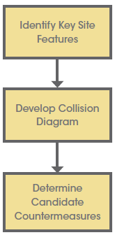
A first step in conducting a site evaluation is to use collision diagrams to diagnose potential safety issues and prevailing crash types at a location.

A diagram that shows the intersection/roadway alignment with the crashes superimposed is known as a collision diagram. This diagram typically includes relevant information including type and severity of crash, date and time of crash, weather, and lighting conditions. Plotting the general crash location and associated information can help to highlight crash trends, if present. The following steps depict this process.

STEP 1: Identify key site features.

An aerial photo or a condition diagram (refer to HSM Figure 5-5, p. 5-7) can be used to identify and document important site characteristics. By inspecting the aerial imagery for this location, one sees that there is a directional median opening that allows left-turns into the driveway, but restricts vehicles exiting the driveways to a right-turn only.

STEP 2: Develop the collision diagram.

The historical (observed) crash data can be used as the basis for developing the collision diagram. The following collision diagram shows the study site crashes for the three-year period.

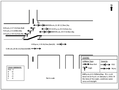
This location predominantly experienced angle and rear-end crashes. The angle crashes appear to be due to the conflict between the left-turning vehicles and the opposing through vehicles at the unsignalized entrance on the north side of the road. These crashes could be a result of restricted sight distance, sun glare issues, or high total intersection volumes with few gaps in traffic. Two of these crashes occurred during rainy conditions. The rear end crashes could be associated with large traffic volumes (and potentially queues from a downstream signalized intersection) or similar issues.

STEP 3: Identify potential countermeasures.

Prior to the field inspection and study by the analyst, it is helpful to explore potential treatments for future mitigation of issues. For the crashes observed at this site, example candidate countermeasures may include:

• Installation of traffic signals (refer to the Manual on Uniform Traffic Control Devices).
• Adjustment of upstream or downstream signal timing to allow progression or to create longer gaps.

Findings

Interpreting the Results:

This simple analysis method used collision and condition diagram techniques to identify specific crash types, prevailing conditions, and potential contributing factors. At this location, eight crashes occurred over a 3-year period. Four of the eight crashes included at least one injury. Based on the collision diagram, it appears that suitable countermeasures will target rear-end and angle crashes; however, due to the small number of crashes the analyst may want to assess how crashes at this location are comparable to crashes at similar locations in an effort to determine whether this location merits improvement at this time.

Possible Errors to Avoid:

The crash data for this site spanned a period of 3 years. It is recommended that analysts gather data from at least 3 to 5 years of crashes to avoid drawing conclusions that do not accurately reflect the crash history. On a cautionary note, for locations with a limited number of observed crashes, the analyst should not attempt to draw definitive conclusions without extending the analysis to similar sites or by comparing the number of crashes to how many would be predicted for the specific facility using intermediate or advanced safety assessment methods.

Alternative Analysis Approaches:

The Historical Crash Data Evaluation safety assessment methods can also be used to supplement this analysis. If the analyst determines that there is sufficient justification to extend the assessment to a detailed evaluation of the candidate location, the next step would be to acquire specific site characteristic information. This added information would then enable the analyst to predict crashes (using the SPF with CMF Adjustment procedure). The predicted number of crashes represents an estimate of how many crashes are typically observed for facilities with similar traffic volumes and roadway characteristics. This additional comparison will strengthen the analysis and help clarify if the location has more crashes than similar locations.

2.3 Justifying the Need for Potential Cost-effective Safety Countermeasures for a Rural Two-lane Highway

Problem Overview

• Safety Assessment Method: CMF Applied to Observed Crashes and CMF Relative Comparison
• Project Phase: Planning & Scoping
• Project Type: 2R
• Related Task: Establish Project Scope
• Calculation Method: Hand Calculated
• Comments: This example problem shows how a basic analysis can be used to identify potential countermeasures that will reduce crashes.

Level of Analysis

Note: See table 3 for a full definition of Project Type designations.

Problem Description

As part of the planning and scoping activities, a roadway agency has identified a 10-mile section of rural two-way, two-lane highway targeted for safety improvements. Many of the crashes appear to be due to vehicles running off of the road. In the most recent 3 years, almost 40 crashes have occurred within this 10-mile section of highway. During the diagnosis process, the roadway agency identified potential treatments that included removal or relocation of fixed objects, installation of center line rumble strips, and delineation of obstacles. The associated Project Type is 2R and the Related Task is to Establish Project Scope. How can the analyst estimate the safety performance of previously identified candidate low-cost countermeasures?

Summary of Available Data:

The following data describes the current conditions and associated crash data.

• Two-lane, two-way operation with lane widths of 11 ft.
• No paved or graded shoulders.
• Average annual daily traffic (AADT) 1,723 vehicles per day (vpd).
• Rolling terrain with numerous horizontal curves.
• Average side slope 1V:3H (1 ft. vertical for every 3 ft. horizontal).
• Three-year crash count = 38 total.
  • Two fatal.
  • Nine injury crashes.
  • Twenty-seven PDO crashes

The crash data currently does not include extensive detail about the individual vehicle maneuvers for each crash, and so the analyst will focus on total crashes and crash severity for this evaluation.

Analysis

Selecting Appropriate Safety Assessment Method(s):

The roadway agency can evaluate the candidate safety assessment methods shown in Table 5. The purpose for this analysis is to use the crash information to assess what types of improvements can be implemented to help reduce future crashes along the corridor. This task and project type is associated with one of the four Basic safety assessment methods. Since a CMF-based method considers a change in road characteristics, the two candidate safety assessment methods that use CMFs are applicable for this analysis. Both methods can be considered. The CMF Applied to Observed Crashes method can be directly applied to the observed crashes. The estimated future crashes can be compared to historical crash data to evaluate the potential reduction in crashes based on the individual improvements. The cost of the reduced number of crashes can then be quantified by applying the equivalent property damage method of calculating a benefit/cost (B/C) ratio.

The CMF Relative Comparison approach does not explicitly consider historical crashes at the site and so is simply used to compare two candidate improvements.

Linkage to the HSM:

Chapter 6 of the HSM (Section 6.2.2, pp. 6-3 to 6-9) summarizes contributing factors to consider when selecting appropriate countermeasures. Section 6.3 of the HSM (p. 6-9 to 6-10) provides guidance for selecting potential countermeasures. Finally, Part D (Volume 3) of the HSM and the FHWA sponsored CMF Clearinghouse (www.cmfclearinghouse.org) include a wide variety of potential improvements. These CMF resources identify the base conditions and applicable site applications for the individual countermeasure of interest.

Detailed Analysis:

Method 1: CMF Applied to Observed Crashes

The analyst will evaluate the candidate treatments recommended as a result of the site diagnosis. There are many potential improvements designed to help mitigate run-off-the-road crashes, but this detailed analysis focused on the three low-cost options.

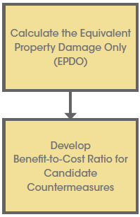
The following steps review the use of the equivalent property damage only (EPDO) performance measure to first identify the value of the crashes and then the CMF Applied to Observed Crashes safety assessment method to further evaluate how the low-cost improvements may help to reduce crashes. A benefit/cost (B/C) ratio can then be used to assess which treatments would be the most cost effective.

STEP 1: Calculate the EPDO value for existing crashes.

The HSM provides sample weighting factors to calculate the EPDO (HSM Table 4-7, p. 4-29). The roadway agency performing this analysis uses the following cost values and resulting weighting factors; however, the values can vary by agency and so it is recommended that they be confirmed prior to analysis.

Severity	Comprehensive Crash Costs (f(cost))	Weighting Factor Calculation	Weighting Factor (f(weight))
Fatal (K)	$4,008,900	fk (weight) = 4,008,900 / 7,400	542
Injury (A/B/C)	$82,600	finj (weight) = 82,600 / 7,400	11
PDO (O)	$7,400	fPDO (weight) = 7,400 / 7,400	1

Note: A=incapacitating injury. B=serious injury. C=possible injury. PDO = property damage only.

The EPDO weighting factors are then applied to the individual crash severity frequencies to calculate the equivalent number of property damage only (PDO) crashes.

Total EPDO Calculation	Notes
=fk(weight) (N(observed,k))+finj(weight) (Nobserved,inj) + fPDO(weight) (Nobserved,PDO)	None.
=(542)(2)+(11)(9)+(1)(27)=1210	The makeup of the existing crashes (all severity levels) is equivalent to having 1210 PDO crashes.

Note: EPDO = equivalent property damage only. PDO = property damage only.

STEP 2: Calculate the B/C ratio of the candidate treatments.

For this evaluation, the analyst is considering improving the clear zone (removing roadside obstacles and trees), adding center line rumble strips, or delineating obstacles where appropriate. The following summary presents these three low-cost treatment options and information related to the cost and effectiveness of each.

Proposed Treatment	Estimated Cost (for 10-mile segment)	CMF (S.E.)1	Crash Type (Base Condition)	Crash Severity	Source
Remove or relocate fixed objects outside of clear zone	$200,000	0.62 (0.103)	★★★ All crash types and roadway types	All	http://www.cmfclearinghouse.org/detail.cfm?facid=1024
Install center line rumble strips	$30,000	0.91 (0.02)	★★★★★ All crash types and rural roadway types	All	http://www.cmfclearinghouse.org/detail.cfm?facid=3361
Delineate obstacles	$10,000	1.0 (0.1)	All crash types and roadway types	All	The HSM CMF value is 1.0. Because CMFs are multiplicative, a value of 1.0 has no effect on crash reduction for these crash types.

_{¹S.E. refers to the standard error
★ CMF Clearinghouse Star Rating.
Note: CMF = crash modification factor. HSM = Highway Safety Manual.}

For these potential improvements, the crash type is the "all" or total crash category. Many of the available CMF values focus on run-off-road crashes. Since this level of information is not available for the study site, the analyst must check to be sure that the correct CMF base conditions are applicable to the study site. For these three specific proposed treatments, the CMFs do apply to "All" crashes and not just to run-off-road collisions. Whenever the data is available, a preferred CMF comparison would be to evaluate the target crashes by type for each CMF. This requires information about the individual crash types at the site as well as CMFs that have the crash type base condition of interest. For this calculation, the target crash level of detail is limited (thus the "all crash type" approach). Using the Total EPDO in Step 1 as a baseline, apply the CMF to calculate the estimated EPDO for each potential treatment.

Remove or relocate fixed objects outside of clear zone:

Calculations	Notes
Estimated EPDO= Total EPDO×CMF=1210×0.62=750.2	-
Cost of Existing EPDO= 1210×$7,400=$8,954,000	This is the estimated cost of the existing crashes on the roadway.
Cost of Estimated EPDO= 750.2×$7,400=$5,551,480	This is the estimated cost of the future crashes for a similar time period if this treatment is selected
B/C Ratio = Cost of Existing EPDO-Cost of Estimated EPDO / Cost of Treatment B/C Ratio = ($8,954,000-$5,551,480)/$200,000 = 17.0	This indicates that the benefits outweigh the cost of the countermeasure (for every $1 the agency spends there is an equivalent benefit of $17).

Install center line rumble strips:

Calculations	Notes
Estimated EPDO = 1210×0.91=1101.1	-
Cost of Existing EPDO = 1210×$7400=$8,954,000	This is the estimated cost of the existing crashes on the roadway
Cost of Estimated EPDO = 1101.1×$7400=$8,148,140	This is the estimated cost of the future crashes on the roadway if this treatment is selected
B/C Ratio = ($8,954,000-$8,148,140)/$30,000 = 26.9	This indicates that the benefits outweigh the cost of the countermeasure (for every $1 the agency spends there is an equivalent benefit of $27).

Delineate obstacles:

Calculations	Notes
Estimated EPDO = Total EPDO×CMF=1210×1.0=1210	–
Cost of Existing EPDO = 1210×$7400=$8,954,000	This is the estimated cost of the existing crashes on the roadway. (same as the other treatments)
Cost of Estimated EPDO = 1,210×$7400=$8,954,000	This is the estimated cost of the future crashes on the roadway if this treatment is selected.
B/C Ratio = ($8,954,000-$8,954,000)/$10,000 = 0.	This indicates that there is no real financial benefit for choosing this countermeasure if the objective is to target all crash types.

Based on the resulting B/C ratios, the analyst concludes that the recommended treatments, in order of priority, should be:

1. Install center line rumble strips (B/C ratio of 26.9), and then
2. Remove or relocate fixed objects outside of the clear zone (associated with a B/C ratio of 17.0).

The analyst eliminates the delineate obstacles option because it has a B/C ratio of 0.0, indicting no real financial benefit.

Method 2: CMF Relative Comparison

The CMF Relative Comparison safety assessment method can be used to compare potential CMFs to evaluate which have the greatest impact on reducing crashes. Whereas in the previous CMF Applied to Observed Crashes calculations, the analyst used observed crash data as a key input into the analysis, only the CMF information is required for the relative comparison approach.

STEP 1: Review the three CMFs previously identified and compare their relative values. The information for the three previously reviewed CMFs is summarized in the following table. Recall that a CMF value less than 1.0 is associated with a larger reduction in future crashes when compared to a CMF with a value of one (assumed to have no real effect on reducing crashes). Based on this simple comparison, the analyst concludes that the recommended treatments, in order of priority, should be:

1. Remove or relocate fixed objects outside of the clear zone (associated with an estimated 38 percent reduction in crashes), and then
2. Install center line rumble strips (associated with a 9 percent estimated crash reduction).

For the purposes of reducing crashes, the analyst removes delineating obstacles from consideration.

Proposed Treatment	CMF (S.E.)1	Crash Type (Base Condition)	Crash Severity
Remove or relocate fixed objects outside of clear zone	0.62 (0.103)	★★★ All crash types and roadway types	All
Install center line rumble strips	0.91 (0.02)	★★★★★ All crash types and rural roadway types	All
Delineate obstacles	1.0 (0.1)	All crash types and roadway types	All

¹S.E. refers to the standard error.
★CMF Clearinghouse Star Rating.
Note: CMF = crash modification factor. HSM = Highway Safety Manual.

Findings

Interpreting the Results:

Based on the low-cost improvements considered using Method 1, the analyst concluded that the center line rumble strips and clear zone improvements provide evidence that the societal benefit of installing the treatments will outweigh the cost of installation. Other considerations may include whether there are any ordinances that limit where rumble strips can be installed. Because this evaluation targeted all crash severities and all crash types, the effect of countermeasures specifically expected to reduce roadside crashes may not be clear.

The Method 2 approach similarly identified the same two CMFs, but did not directly consider crash data, weighting of severity levels, or benefit/cost analysis. This relative comparison approach, based simply on anticipated treatment effectiveness, prioritized the clear zone improvements above the center line rumble strips. This more basic approach provided useful information, but did not include site-specific information required for Method 1.

Possible Errors to Avoid:

It is recommended that analysts utilize crash cost estimations and weighting based on their State or local crash cost databases. Appropriate CMFs used for this type of analysis will have crash type and base condition characteristics that match those of the project highway.

Alternative Analysis Approaches:

The two methods may be effective approaches to initially narrow down the large list of potential safety treatments. If additional data that includes individual road geometry and crash type could be acquired for this location, a more comprehensive evaluation based on predicted or expected crashes could be performed during the preliminary and final project development phases.

2.4 Predicting Crashes to Evaluate Level of Service of Safety for a Rural Two-lane Highway

Problem Overview

• Safety Assessment Method: SPF with CMF Adjustment
• Project Phase: Planning & Scoping
• Project Type: 3R
• Related Task: Establish Project Scope
• Calculation Method: Tool Calculated
• Comments: This example problem calculates the predicted number of crashes for alternative curve geometry options along a rural two-lane highway and then applies a level of service of safety ranking.

Level of Analysis

Note: See table 3 for a full definition of Project Type designations.

Problem Description

As part of planning and scoping activities, a DOT is developing plans to resurface a seven-mile section of a rural two-lane highway that contains 13 horizontal curves. The analyst wants to ensure that any low-cost curve countermeasures deployed as part of this project will have a positive impact on reducing crashes. The DOT does not have information about the roadside hazard rating or the driveway access density for each curve, and so the analyst visually inspected several of the curve locations and developed an average value to use for these road characteristics during this preliminary analysis phase. The associated Project Type is 3R and the Related Task is to Establish Project Scope. How can the analyst estimate which curves are functioning as anticipated and which ones could benefit from low-cost treatments?

Summary of Available Data:

The relevant curve characteristics include the following for all 13 curves:

• AADT = 10,250 vpd (Curves #1 through #11), AADT = 9,700 (Curves #12 and #13).
• Lane width = 11 ft.
• Paved shoulder width = 6 ft. (right and left shoulders).
• No spiral transitions.
• Superelevation at curves compatible with design values.
• Level grade.
• No center line rumble strips, passing lanes, or two-way left-turn lanes.
• Driveway density = 5 driveways/mi (estimated average).
• Roadside hazard rating = 3 (estimated average).

The individual curve characteristics are further described as follows:

Curve Number	Delineation Devices Present	Length (mi)	Radius (ft)	Superelevation rate (percent)	3-Year Total Crash Count
1	None	0.25	1229	4.7	7
2	None	0.26	1269	5.5	3
3	Chevrons	0.12	384	7.8	1
4	Delineators	0.08	588	3.1	2
5	None	0.09	629	3.1	1
6	None	0.19	750	6.2	1
7	None	DATA_HERE	DATA_HERE	DATA_HERE	DATA_HERE
8	Delineators	0.06	309	7.0	5
9	None	0.05	818	6.2	0
10	Delineators	0.15	794	9.4	1
11	Chevrons	0.17	678	3.9	2
12	Chevrons	0.22	706	3.9	0
13	None	0.15	800	7.8	1

_{Note that total crash count information is currently the only available crash data.}

Analysis

Selecting Appropriate Safety Assessment Method(s):

The analyst must first review the potential safety assessment methods shown in Table 5 for 3R project types and the task of establishing the project scope. This task and project type is associated with the four Basic and the two Intermediate safety assessment methods. For this analysis, the DOT only has limited funds available for select curve improvements. The analysis needs to include enough detail to evaluate the individual curves so that the limited funds are targeted effectively. Note that an intersection located between curves #11 and #12 results in different (lower) traffic volumes for the last two curves.

Of the four Basic methods, only the CMF-related safety assessment methods can directly consider horizontal curve radius, but the two basic CMF-related methods do not consider the varying traffic volume. For the two Intermediate safety assessment methods, the SPF with CMF Adjustment safety assessment method can also evaluate the horizontal curve geometry. The AADT-Only SPF safety assessment method does not consider varying geometric characteristics and can be eliminated as a candidate for this analysis.

The SPF with CMF Adjustment will allow an evaluation of the different curve radii as well as varying traffic volume for the last two curves. This method also results in predicted crash information as noted in Table 1. To most effectively use this approach, an agency should calibrate the SPF for their local jurisdiction. A calibration factor of 1.0 can be used if this information is not available, but the results will not be refined to local conditions.

Once predicted crashes are calculated, a variety of analysis approaches can be used to then determine which curves merit additional treatment. For this assessment, the analyst will calculate the predicted crash frequencies and then compare these frequencies to the observed crash frequencies by applying the measure of Level of Service of Safety (LOSS).

Linkage to the HSM:

The HSM can be used to estimate the number of predicted crashes for a rural, two-lane highway by applying the procedures introduced in HSM Chapter 10 (pp. 10-1 to 10-74). By determining predicted crashes, the analyst can estimate how many crashes may be expected for a specific road type with varying road conditions (in this case the curve radii and traffic volumes). The HSM provides manual calculations, but a spreadsheet tool is available and can be used to simplify this analysis.

Once the number of predicted crashes has been calculated, the predicted crashes can be compared to the historical (observed) average crash frequency to identify which curves have diminished levels of service of safety (LOSS) that merit additional consideration. This LOSS procedure is reviewed on p. 4-12 of the HSM. An example problem is included on pp. 4-44 to 4-48 of the HSM.

Detailed Analysis:

The following steps provide the calculations for predicting rural two-lane highway crashes based on using the HSM "Smart Spreadsheets" available for download at: http://www.highwaysafetymanual.org/Pages/tools_sub.aspx#4. For this example problem, the analyst can use the "HSM prediction rural two-lane roads" spreadsheet tool.

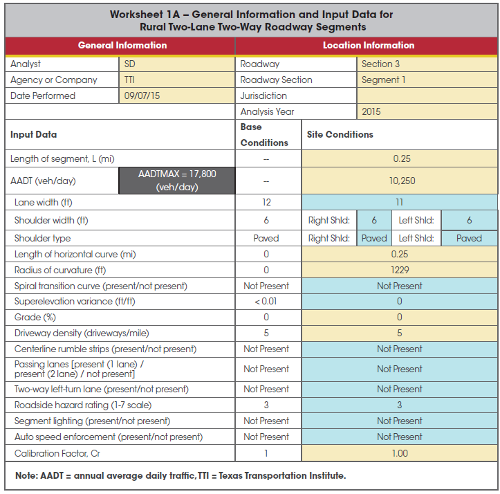
STEP 1: Input the data describing each curve into the spreadsheet tool.

Note that no lighting or automated speed enforcement is present. The following graphic shows a representation of Worksheet 1A. This roadway segment worksheet includes input information similar to that shown in the HSM worksheet (see HSM p. 10-68). The input data shown in the graphic represents data cells for the first curve on the highway section (radius of 1229 ft).

STEP 2: Tabulate the predicted crash frequency for each curve and convert the frequencies to predicted 3-year crash counts.

The following graphic shows a representation of Worksheet 1C. This roadway segment worksheet summarizes the predicted crash frequency for each year. The values shown represent segment #1. This worksheet includes input information similar to that shown in the HSM worksheet (see HSM p. 10-69).

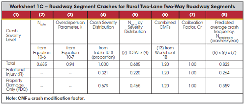
The total predicted numbers of crashes per year, the equivalent total predicted crashes for 3 years, and the observed 3-year crash frequency are shown in the following table. The 3-year predicted crash count for Curve #1 is calculated as 2.47 (= 0.823 crashes/year × 3 years). Upon inspection of the crash values, the design team notes that Curves #1, 2, 4, 7, and 8 all have more observed crashes than were predicted for a road of this type with similar volume and curve radii characteristics, though when compared to rounded predicted crashes, only Curves #1 and #8 have observed crashes that are noticeably higher. Additional evaluations can help determine if these five curve locations should be the final improvement curves. This evaluation is included in Step 3.

STEP 3: Use the crash counts to compute the level of service of safety procedure described in HSM Section 4.4.2.7 (HSM pp. 4-44 to 4-48).

The level of service of safety is based on assessing the amount of deviation between the predicted and the observed crashes. To calculate the LOSS, the curves are separated into four categories (I to IV). Sites with a moderate to high potential for crash reduction (or LOSS category rankings of III or IV) are then identified for future study.

Curve Number	Predicted Crashes			Observed Crash Total for 3 years
	Calculated Total for 1 Year	Total for 3 years
		Calculated	Rounded
1	0.823	2.47	3	7
2	0.847	2.54	3	3
3	0.718	2.15	3	1
4	0.473	1.42	2	2
5	0.485	1.46	2	1
6	0.730	2.19	3	1
7	0.355	1.07	2	2
8	0.641	1.92	2	5
9	0.319	0.96	1	0
10	0.606	1.82	2	1
11	0.694	2.08	3	2
12	0.782	2.35	3	0
13	0.572	1.72	2	1

The LOSS category criteria are summarized as follows:

Category I: σ < N_observed < (N – (1.5 × σ)) [Low potential for crash reduction].

Category II: (N – (1.5 × σ))≤ N_observed ≤ N [Low to moderate potential for crash reduction].

Category III: N ≤ N_observed ≤ (N + (1.5 × σ)) [Moderate to high potential for crash reduction].

Category IV: Nobserved ≥ (N + (1.5 × σ)) [High potential for crash reduction].

For these classifications, the standard deviation, σ, is calculated as follows (Equation 4-16 of the HSM):

Where:

• k represents the overdispersion parameter of the SPF (this specific SPF has a value of 0.236 ÷ L as noted in the HSM equation 10-7, p. 10-16).
• N represents the predicted crash frequency.
• L represents the length of roadway segment in miles.

The following summary table identifies the individual LOSS rankings for the 13 curve locations. The shaded curves are the same five curves identified during the Step 2 evaluation. All five curves have LOSS category classifications of III and IV, suggesting that they are the curves that merit attention.

As an example, the standard deviation (σ) for Curve Number 1 is calculated as follows:

The four potential LOSS category classifications can then be evaluated. As an example, the LOSS assessment for Curve Number 1 is calculated as follows:

Category I Assessment – Curve #1:

Is σ < N_observed < (N – (1.5 × σ))?

Is 2.40 < 7 < [(2.47 – (1.5 × 2.4)) = -3.6]?

No, 7 is not less than -3.6, so proceed to evaluate Category II.

Category II Assessment – Curve #1:

Is (N – (1.5 × σ) ≤ Nobserved ≤ N?
Is [(2.47 – (1.5 × 2.4)) = -3.6] ≤ 7 ≤ 2.47?
No, 7 is not less than 2.47, so proceed to evaluate Category III.

Category III Assessment – Curve #1:

Is N ≤ N_observed ≤ (N + (1.5 × σ))?
Is 2.47 ≤ 7 ≤ [(2.47 + (1.5 × 2.40)) = 6.07]?
No, 7 is not less than 6.07, so proceed to evaluate Category IV.

Category IV Assessment – Curve #1:

Is N_observed ≥ (N + (1.5 × σ))?
Is 7 ≥ [(2.47 + (1.5 × 2.40)) = 6.07]?
Yes, so Curve #1 has a Category IV LOSS.

Curve Number	Predicted 3-Year Crash Count	Observed 3-Year Crash Count	σ	Level of Service of Safety
1	2.47	7	2.40	IV
2	2.54	7	2.40	III
3	2.15	1	3.02	II
4	1.42	2	2.44	III
5	1.46	1	2.36	II
6	2.19	1	2.44	II
7	1.07	2	1.84	III
8	1.92	5	3.81	III
9	0.96	0	2.09	II
10	1.82	1	2.28	II
11	2.08	2	2.45	II
12	2.48	0	2.57	II
13	1.82	1	2.28	II

Findings

Interpreting the Results:

The results of the level of service of safety analysis show that there is a high potential for crash reduction (i.e. LOSS Category of IV) on Curve #1 and a moderate-to-high potential for crash reduction (i.e. LOSS Category III) for Curves #2, #4, #7, and #8. These curves are candidates for additional crash reduction treatments. The simple comparison between rounded predicted values and observed crashes, however, further indicates that Curves #1 and #8 merit priority attention.

Possible Errors to Avoid:

When using the HSM predictive method, the input value for superelevation differential can be confusing. The value used in the procedure is for a difference (in ft. per ft) of how the existing superelevation slope deviates from the design slope. As an example, if the proposed superelevation design value for a curve is 4.80 percent but instead the actual slope is 2.20 percent, the deviation would be calculated as: 0.048 -0.022 = 0.026. For this evaluation, there were not any superelevations variances of significance, and so this value would be 0.00.

Alternative Analysis Approaches:

The analyst could have used the CMF Applied to Observed Crashes safety assessment method to compare Curves #1 through #11 since they all had the same traffic volume. A separate, similar analysis for Curves #12 and #13 could also be performed. The result of this procedure, however, provides estimated crashes (instead of predicted crashes that are calculated when using an SPF). LOSS is one of several measures that are presented in Chapter 4 of the HSM for use in planning and programming highway improvements that can reduce crash frequency or severity. As shown in Table 6, an alternative performance measure that also uses SPF information as it applies to contrasting predicted crashes is the Excess Predicted Average Crash Frequency Using SPFs.

Expected crashes can also be considered for comparing site-specific conditions prior to making substantial changes. As the project shifts from the planning stage to the design stage, these more detail-oriented procedures may be appropriate as they can prove to be particularly useful as input into benefit/cost analyses during the final stages of the project.

2.5 Predicting Incremental Benefits Associated with Increased Lane Width for a Rural Two-lane Highway

Problem Overview

• Safety Assessment Method: SPF with CMF Adjustment
• Project Phase: Planning & Scoping
• Project Type: 3R
• Related Task: Establish Project Scope
• Calculation Method: Tool Calculated
• Comments: This example problem will evaluate the effect lane widening can have on reducing fatal and injury crashes for a two-lane undivided rural highway at a site where crash data is not available.

Level of Analysis

Note: See table 3 for a full definition of Project Type designations.

Problem Description

A two-lane county highway serving a newly developed residential community is in need of some upgrades. Currently, the two-lane highway has 10-ft. lanes and the road does not have any graded or paved shoulders (a typical rural low-volume design at the time it was constructed). The county has funding limitations but intends to widen the travel lanes as a short-term solution to help improve corridor operations. The analyst would also like to evaluate safety estimates and compare the added incremental benefits of widening the lanes from 10-ft. to 11-ft. wide and from 10-ft. to 12-ft. wide. A specific goal would be to evaluate how these improvements would reduce the number of fatal or injury crashes annually along this corridor. A future project could also consider adding graded shoulders, but due to limited funding, this option must be deferred to a later date. The affected corridor is approximately 20 miles long with a current AADT of 10,000 vpd. The Project Type is 3R and the Related Task is to Establish Project Scope. How does the analyst estimate the reduction in the number of fatal and injury crashes due to these potential incremental improvements?

Summary of Available Data:

The County does not have any available crash data for this corridor. To simplify this initial assessment, the analyst has made the following assumptions:

• No horizontal curves.
• No vertical grades steeper than 2 percent.
• Driveway density of five driveways per mile.
• No center line rumble strips, passing lanes, or two-way left turn lanes.
• Roadside hazard rating of three.
• No street lights.
• No automated speed enforcement.

Analysis

Selecting Appropriate Safety Assessment Method(s):

Based on Table 5, the Establish Project Scope task and the 3R project type are associated with the four Basic and the two Intermediate safety assessment methods. There is limited data available for the corridor and the goal is to estimate the reduction in fatal and injury crashes due to incremental widening. Because this condition eliminates methods that only evaluate existing conditions (see Table 1 in Chapter 1), the Site Evaluation or Audit and the Historical Crash Data Evaluation safety assessment methods are not applicable. In addition, the CMF Applied to Observed Crashes is also not feasible due to the lack of available crash data. The AADT-Only SPF method does not explicitly allow evaluation of unique road features and so this method also does not apply.

The remaining potential safety assessment methods include CMF Relative Comparison and SPF with CMF Adjustment. The relative comparison method can be used if CMFs are available for the proposed lane widening.

The analyst conducts a quick search on the FHWA CMF Clearinghouse (http://www.cmfclearinghouse.org/) to determine if CMFs are available for the widening scenario (i.e., widen lane from 10 ft. to 11 ft., widen lane from 10 ft. to 12 ft.). Note that the base condition would be 10 ft. lane widths for the two options. In addition, the lane width CMFs that the analyst does locate do not provide information about the number of fatal or injury crashes. Based on this assessment, the analyst concludes that the SPF with CMF Adjustment method appears to be the preferred safety assessment method for this evaluation.

Linkage to the HSM:

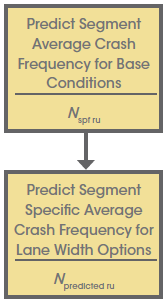
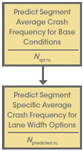
The HSM can be used to estimate the number of predicted crashes for a rural, two-lane highway by applying the procedures introduced in HSM Chapter 10 (pp. 10-1 to 10-74). By determining the predicted total, fatal and injury, and property damage only crashes for the 10 ft, 11 ft, and 12 ft. lane scenarios, the analyst can assess the incremental benefits associated with the lane widening options. The HSM provides manual calculations, but a spreadsheet tool is available and can be used to simplify this analysis.

Detailed Analysis:

The analyst reviews the criteria for the SPF with CMF Adjustment safety assessment method and notes that the SPF from the HSM has not been calibrated for the region. Therefore, the analyst can simply use a calibration factor value of 1.0. Because the evaluation compares lane-width options for the same facility, the absence of a calibration factor for the region will not adversely affect the process of comparing design options for the same road. The predicted number of crashes may not be exact, but the procedure can accurately calculate the relationship between the predicted numbers of crashes for varying lane widths. Due to the absence of a calibrated SPF, the analyst will report the results as a percentage reduction in crashes instead of a specific number of reduced crashes. This reporting format is appropriate because reporting the number of crashes would imply more precision than the calculations (that do not incorporate a calibration factor) represent.

The following steps provide the calculations based on using the HSM "Smart Spreadsheets" available for download at: http://www.highwaysafetymanual.org/Pages/tools_sub.aspx#4. For this example problem, the analyst can use the "HSM rural two lane roads" spreadsheet tool.

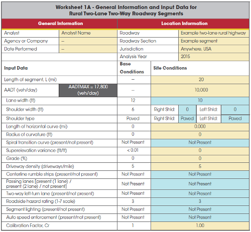
STEP 1: Input the data describing each lane width option into the spreadsheet tool.

As previously indicated, the analyst used a calibration factor of 1.0. She also included the base conditions for each feature, a volume of 10,000 vpd, and length of 20 miles. The following graphic shows Worksheet 1A. This roadway segment worksheet includes input information similar to that shown in the HSM worksheet (see HSM p. 10-68). The input data shown in the graphic represents data cells for the 10-ft.-lane-width option (existing conditions).

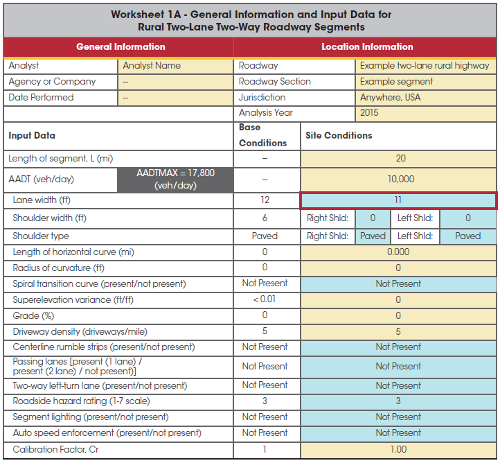
This analysis can be repeated for the 11-ft. and the 12-ft. lanes by changing the lane width field value. The input data for the 11-ft. alternative is shown with the applicable field outlined in red.

STEP 2: Tabulate the predicted crash frequency for each lane width option.

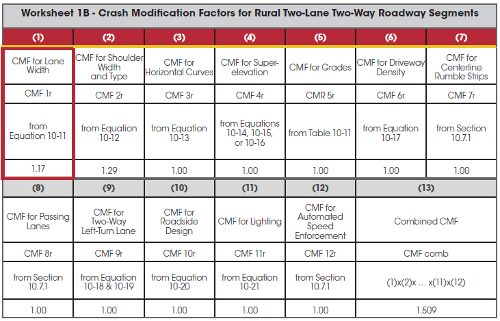
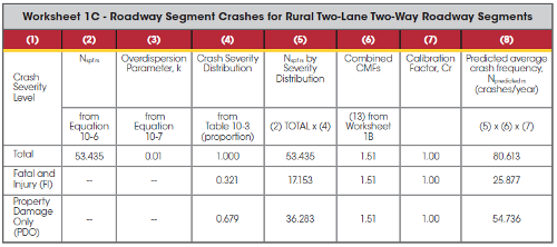
Following input in Step 1, the spreadsheet tool automatically calculates the predicted number of crashes. To review the example results for the segment calculations, see the CMF results for the Existing Condition (shown in Worksheet 1B with the lane width CMF outlined in red) and predicted number of crashes (Worksheet 1C). These roadway segment worksheets are similar to the HSM worksheets with the same numbering format (see HSM p. 10-69).

 

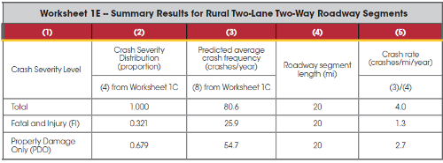
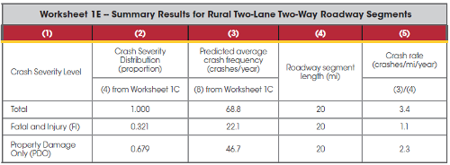
The summary results are shown in Worksheet 1E (see HSM p. 10-70). The segment analysis results for the Existing Condition are shown below. These values are used in Step 3.

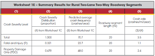
The results for the 11 ft. lane width alternative (Worksheet 1E) are shown below.

The results for the 12 ft. lane width alternative (Worksheet 1E) are shown below.

STEP 3: Summarize the total number of crashes.

The analyst next created the following table that summarizes the total number of predicted crashes per year for the three scenarios (based on the assumed calibration factor of 1.0).

Alternative	Predicted Crashes per Year (Npredicted)
	Total	Fatal and Injury	Property Damage Only
10-ft. Existing Lanes	80.6	25.9	54.7
11-ft. Lane Alternative	70.7	22.7	48.0
12-ft. Lane Alternative	68.8	22.1	46.7

The spreadsheet values do not include any rounding errors as would be expected when performing calculations by hand. As a result, these numbers will be similar, but may not exactly match predicted crashes calculated manually.

STEP 4: Summarize the total reduction in fatal and injury crashes. The analyst's ultimate goal is to evaluate if the reduction in the number of fatal and injury crashes due to widening the lanes from 10 ft. to 11 ft., which would be substantially different from widening the lanes from 10 ft. to 12 ft. The following table summarizes this analysis.

Roadway Improvement Scenario	Number of Predicted Fatal and Injury Crashes per year		Predicted Reduction in the Number of Fatal and Injury Crashes	Reduction in the Number of Fatal and Injury Crashes
	Existing Width	Final Width
Widening lanes from 10 to 11 ft.	26	23	3	12
Widening lanes from 10 to 12 ft.	26	22	4	15

Findings

Interpreting the Results:

Based solely on an evaluation of the predicted number of crashes, a road with the characteristics described for the existing configuration can be expected to experience approximately 81 crashes per year, of which about 26 would involve a fatality or injury.

11-ft. Lanes: By adding 1 ft. of pavement to each lane (increasing to 11-ft. lanes), the analyst can expect to see an approximate 12 percent reduction in fatal and injury crashes per year.

12-ft. Lanes: Adding 2 ft. of pavement to each lane to create 12-ft. lanes leads to a predicted reduction of approximately 15 percent for fatal and injury crashes.

Based on these findings, the analyst concludes that widening lanes from 10-ft. to 12-ft. lanes will result in a 2 to 3 percent additional benefit when compared to widening from 10-ft. to 11-ft. lanes.

These calculations do not consider any local aspects of the roadway that may impact the benefits or costs associated with the increased lane widths. They also do not consider potential improvements in operational level of service associated with wider lanes.

Possible Errors to Avoid:

The HSM spreadsheet simplifies the effort associated with using the predictive method. This planning analysis included several assumptions such as no horizontal curves and vertical grades that are two percent or less. The results, therefore, are suitable for comparative purposes but do not represent the final roadway geometric conditions. A more detailed analysis during the design stage would provide additional useful information about predicted crashes.

Alternative Analysis Approaches:

A common method for evaluating design alternatives is to use CMF comparisons that do not directly consider traffic volume. This approach is less reliable than the predictive methods, but can be used to evaluate alternatives when an SPF is not available for the condition. Although the analyst could not locate suitable CMFs for this application, many transportation agencies develop and maintain agency-specific CMFs that could be useful for similar analyses.

prev | next