U.S. Department of Transportation
Federal Highway Administration
1200 New Jersey Avenue, SE
Washington, DC 20590
202-366-4000
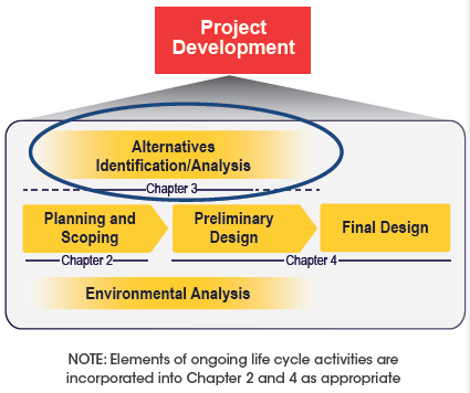
Figure 5. The Project Development Cycle and Corresponding
Alternative Analysis Chapter
The Alternatives Analysis phase is typically conducted after a project need has been determined but before a solution has been identified. This phase may coincide with the Planning and Scoping phase and can extend into the early stages of Preliminary Design. The purpose of safety assessments in the Alternatives Analysis phase is to estimate the impact of each alternative on safety performance.
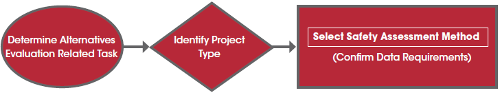
This chapter provides information to help select safety assessment methods suitable for addressing questions related to safety performance that arise during alternatives analysis tasks based upon the related task and project type. This section describes alternatives analysis-related tasks in two general categories:
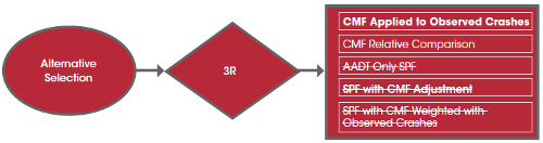
The alternative selection activities generally occur following the preliminary planning activities and may be part of a corridor or project alternatives assessment. The objective of the safety assessment for this task is to estimate the safety performance of alternatives. This information can then be used to help refine the proposed alternatives as the project progresses into the preliminary and final design phases.
New or modified points of access to the Interstate system require Interstate access justification and documentation activities. The Federal Highway Administration's (FHWA) Policy on Access to the Interstate System provides the requirements, which include an analysis of the access point's impact on the safety performance of the Interstate facility and the local street system under both the current and the planned future traffic projections.
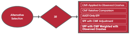
Table 7 identifies the five (out of a possible seven) safety assessment methods generally suitable for lternatives analysis tasks and the objective of the associated safety performance analysis. The check marks in Table 7 suggest suitable safety assessment methods for each related task and objective and, in some cases, are distinguished by project type. In this context, the term "suitable" means that the method generally has the capability to address the objective of the safety performance analysis with the data typically available for the related task and project type.
The following questions illustrate the types of questions the analyst may develop at the beginning of the safety assessment. These questions are based on the example problems included in this chapter.
Table 8 shows that the level of predictive reliability generally increases as the methodology used becomes more complex. At the same time, the required resources for the analysis also will increase. In some cases, it may not be feasible to fully implement the preferred safety assessment method due to limitations in site information, crash data, traffic volume, or similar information. For example, the Basic safety assessment method for a CMF Applied to Observed Crashes cannot be executed if historic crash data is not available.
The approach for selecting a safety assessment method for alternatives evaluation and identification looks like this:
| Related Task | Objective | Project Type | Basic | Intermediate | Advanced | ||||
|---|---|---|---|---|---|---|---|---|---|
| Observed Crashes | CMF Relative Comparison | Predicted Crashes | Expected Crashes | ||||||
| Site Evaluation or Audit | Historical Crash Data Evaluation | CMF Applied to Observed Crashes | AADT-Only SPF | SPF with CMF Adjustment | SPF with CMF Weighted with Observed Crashes | ||||
| Safety Assessments: (Increasing Level of Predictive Reliability from Left to Right) | |||||||||
| Alternative Selection | Estimate the safety performance of alternatives | 2R | ✔ | ✔ | ✔ | ✔ | |||
| 3R, 4R | ✔ | ✔ | ✔ | ✔ | ✔ | ||||
| NL | ✔ | ✔ | ✔ | ✔ | |||||
| Interchange Access Justification | Estimate the safety performance impact of new or modified points of access | 3R, 4R | ✔ | ✔ | ✔ | ✔ | ✔ | ||
| NL | ✔ | ✔ | |||||||
| Data Requirements: Increasing Level of Resources Needed (Staff, Analysis, Time, etc.) from Left to Right | |||||||||
| Road Type1 | ✔ | ✔ | ✔ | ✔ | ✔ | ✔ | |||
| Road Characteristics2 | ✔ | ✔ | ✔ | ✔ | ✔ | ||||
| Traffic Volume (vpd)3 | ✔ | ✔ | ✔ | ||||||
| Observed Crash Data4 | ✔ | ✔ | ✔ | ✔ | |||||
1Road Type refers to rural two-lane highway, rural multi-lane highway, urban freeway, etc.
2 Road Characteristics includes physical features such as lane widths, access density, etc.
3 Traffic Volume is the ADT or AADT in vehicles per day.
4Observed Crash Data represents the historic crash data at the study site for a period of more than one year (preferably 3 to 5 years).
5See Example Problem 3.1.
6 See Example Problem 3.2.
7See Example Problem 3.3.
8See Example Problem 3.4.
9See Example Problem 5.2.
Note: Project type definitions are as follows: R2 = resurfacing existing facilities. R3 = major rehabilitation of an existing facility. R4 = major retrofit construction efforts. NL = highway construction at a new location. See Table 3 for a full definition of each Project Type. ✔ = suitable safety assessment method. ADT = average daily traffic. AADT = annual average daily traffic. CMF = crash modification factor. SPF = safety performance function. vpd = vehicles per day.
This chapter provides examples that demonstrate the selection process for the alternatives analysis safety assessment methods. These examples are simplified hypothetical problems intended to illustrate the thought process for selecting a method and demonstrate how to apply the method to answer the associated safety-based question.
![]()
Note: See table 3 for a full definition of Project Type designations.
Currently, there are three travel lanes in each direction with a two-way left-turn lane. Over the past 5 years there have been a total of 362 injury crashes (72.4 average injury crashes per year) along the 1-mile segment. Fortunately, there have not been any fatal crashes at this location during the study period. The city does not have a current AADT value for this corridor.
The analyst for the city can evaluate the candidate safety assessment methods shown in Table 8 and contrast the table information with the 3R project type and the alternative selection task. There are five potential safety assessment methods for the analyst to consider: two basic, two intermediate, and one advanced. Because this assessment will likely require the use of the injury crash information as input into the evaluation, and the analyst's goal is to calculate the estimated reduction in injury crashes following construction of a raised median or implementation of corridor-specific traffic calming measures, a CMF-based method that accounts for the a change in road characteristics is appropriate. In addition, the city does not have a current AADT value for the corridor, so volume-based methods are not feasible at this time. These constraints result in the elimination of the SPF-based methods.
The two remaining safety assessment methods that use CMFs include CMF Applied to Observed Crashes and CMF Relative Comparison. Both methods can be considered.
The CMF Applied to Observed Crashes method can directly evaluate the proposed road design modification and the observed injury crashes. Using the observed crash injury frequency to represent the existing conditions and then applying an appropriate CMF, the analyst can estimate the average injury crash frequency for the proposed condition. For these reasons, the analyst selected the CMF Applied to Observed Crashes safety assessment method.
The CMF Relative Comparison approach does not explicitly consider the historical (observed) crashes along the corridor, but can be used for simple comparison purposes between the two proposed treatments. (Refer to Problem 2.2 for an example where the analyst elected to apply both methods.)
Chapter 6 of the HSM (Section 6.2.2, pp. 6-3 to 6-9) summarizes contributing factors to consider when selecting appropriate countermeasures. Section 6.3 of the HSM (p. 6-9 to 6-10) provides guidance for selecting potential countermeasures. Finally, Part D (Volume 3) of the HSM and the FHWA sponsored CMF Clearinghouse (www.cmfclearinghouse.org) include a wide variety of potential improvements to consider.
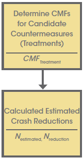
The estimated average crash frequency is calculated by multiplying the appropriate CMF for the alternative treatment by the number of observed crashes that apply to the selected CMF.
STEP 1: Identify CMFs for each treatment
The CMF Clearinghouse (www.cmfclearinghouse.org) and the HSM are two resources for this activity. It is important to confirm that the CMFs have similar crash types and base conditions. The following table shows potential CMFs for the two candidate treatments. The CMF Clearinghouse star rating is based on a scale (1 to 5), where 5 stars represent the highest or most reliable rating. The standard error is one of the rating criteria for the star rating (small standard errors are preferred). The analyst should select CMFs (from the Clearinghouse) with the highest star rating, lowest standard error, and most applicable conditions for the scenario.
| Proposed Treatment | CMF (S.E.) | Setting (Road Type and Traffic Volume) | Crash Severity | Source |
|---|---|---|---|---|
| Treatment – Raised Median | ||||
| Provide a Raised Median | 0.78 (0.02) | ★★★★★ Urban Arterial Multilane (Traffic Volumeunspecified) |
Serious or Minor Injury | HSM Table 13-11, p. 13-14 and http://www.cmfclearinghouse.org/detail.cfm?facid=22 |
| Treatment – Traffic Calming Measures | ||||
| Implement Automated Speed Enforcement Cameras | 0.83 (0.01) | ★★★★★ All Roads (Traffic Volume-unspecified) |
Fatal, Serious Injury, Minor Injury | HSM Table 17-5, p. 17-6 and http://www.cmfclearinghouse.org/detail.cfm?facid=4583 |
Note: AADT = average annual daily traffic. CMF = crash modification factor. HSM = Highway Safety Manual. S.E. = standard error. ★ CMF Clearinghouse Star Rating.
STEP 2: Calculate estimated crash reductions for each alternative.
The following tables contain the calculations for determining the injury crash reductions based on the two individual alternatives. This step can be used to eliminate any treatment combinations that increase the total number of crashes or that have very little effect on the number of injury crashes.
| Calculations | Notes |
|---|---|
| Total Injury Crashes | |
| Nestimated(injury) = CMFRaisedmedian × Nobserved(injury) | Multiply CMF times observed number of injury crashes at location where CMFRaised Median = 0.78 |
| Nestimated(injury) = 0.78 × 72.4 = 56.5 crashes | 362 crashes in 5 years = 72.4 crashes/yr. Approximately 57 injury crashes if this treatment were implemented |
| Nreduction (per year) = 72.4 - 56.5 = 15.9 crashes | Approximately 16 fewer injury crashes each year |
CMF = crash modification factor
| Calculations | Notes |
|---|---|
| Total Injury Crashes | |
| NSestimated(injury) = CMFAutomated Speed Enforcement × Nobserved(injury) | Multiply CMF times observed number of injury crashes at location where CMFAutomated Speed Enforcement = 0.83 |
| Nestimated(injury) = 0.83 × 72.4 = 60.0 crashes | 362 crashes in 5 years = 72.4 crashes/yr Approximately 60 injury crashes if this treatment were implemented |
| Nreduction (per year) = 72.4 – 60.0 = 12.4 crashes | Approimately 12 to 13 fewer injury crashes each year |
CMF = crash modification factor
For this seven-lane arterial, the installation of a raised median is estimated to reduce the total number of injury crashes by approximately 16 per year, equivalent to an approximate 22 percent reduction in injury crashes. The application of automated speed enforcement is similarly estimated to reduce injury crashes but only by 12 to 13 per year (a 17 percent reduction). These findings demonstrate that the raised median will be more effective at reducing injury crashes than the implementation of automated speed enforcement cameras. The safety treatment effectiveness would then be considered in terms of cost to identify the preferred alternative. Because the two treatments target different crash types, the selection of both options may also be preferable for this location.
The selections of CMFs that are not consistent with the conditions of the particular site of interest or the specific target crash type(s) will result in inaccurate estimated average crash frequencies. It is also important to understand that the application of multiple CMFs will not always have a cumulative effect on the estimated average crash frequency. The CMF Clearinghouse FAQ titled "How can I apply multiple CMFs" provides additional information and clarification (see http://www.cmfclearinghouse.org/faqs.cfm#q4).
This analysis focused on injury crashes only and did not consider total crashes. Extending the analysis to other crash types or to crash severity levels could provide additional insights. As previously noted, the use of a relative comparison of CMFs is an additional analysis that can be conducted with the available data. In addition, alternative evaluations could include an economic appraisal such as the benefit/cost ratio or a prioritization evaluation that uses an incremental benefit/cost ratio.
For this study, the city did not have current AADT information. It is feasible, however, that a reasonably accurate traffic volume estimate could be developed based on a combination of traffic volumes from prior years, development trends in the region, and use of comparison sites for volume estimation purposes. As the project shifts from the alternative analysis to the design phase, the analyst will assemble more detailed site-specific data including additional road characteristics. At that time, additional analysis procedures that incorporate CMFs, SPFs, or both can strengthen the overall analysis.
![]()
Note: See table 3 for a full definition of Project Type designations.
A transportation analyst is finalizing the alternative evaluations for a four-lane undivided rural highway. The corridor has a two-way, stopcontrolled intersection with a design speed of 50 mph and relatively little skew. Since about as many vehicles turn into the intersection as turn out of the intersection, the AADT is approximately 30,000 vpd on the major road (upstream and downstream of the intersection) and 5000 vpd on the minor road. The analyst is considering a lowcost redesign option that could be implemented within the currently proposed pavement limits. The change would apply to the roadway cross section that is designed to have 12-ft. inside lane widths, 13-ft. outside lanes, and 8-ft. paved shoulder widths. The analyst wants to identify a prospective lane configuration that will contribute to reducing the number of crashes at this intersection. He has identified two candidate left-turn lane alternatives to evaluate. The Project Type is 2R and the Related Task is Alternative Selection for this effort. How can the analyst compare the estimated crash frequency with Alternative #1, Alternative #2, and the existing configuration?
The segment length that is influenced by the intersection can be assumed to extend approximately 1,000 ft. upstream and 1,000 ft. downstream of the intersection (measured from the intersection center line). This results in a total segment length of approximately 0.38 miles (or two approach segments of 0.19 miles each). Site features include:
The schematic depicts the existing and two potential alternative lane configurations. As noted previously, the corridor is a four-lane rural, multilane, undivided highway with a two-way stop control (on the minor legs). At this time, historical crash data is not available for the existing intersection.
The analyst can first review the potential safety assessment methods shown in Table 8. The Alternative Selection task and the 2R project type are associated with two basic and two intermediate methods. For this assessment, the analyst intends to compare the number of estimated crashes for two alternative intersection lane configurations and contrast these values to the number of estimated crashes for the current intersection approach. Since a CMF-based method enables the specific consideration of a change in road characteristics, the safety assessment methods that use CMFs are applicable for this analysis. Traffic volume information is also available for the major and minor road, and so a safety assessment method that is volume-based can be used. Based on these considerations, the AADT-Only SPF method can be eliminated from further consideration since it does not directly capture changes in road characteristics. As previously noted, the historical (observed) crash data is not currently available for this location, so the CMF Applied to Observed Crashes method should also be eliminated.
The two remaining safety assessment methods include CMF Relative Comparison and SPF with CMF Adjustment. The analyst may elect to use one or both of these methods. The ability to directly incorporate the traffic volume into the analysis, however, strengthens the evaluation, so the analyst elects to use the SPF-based method. Because the data requirements are not substantially different for the CMF Relative Comparison option, this method could be an effective way to narrow down candidate lane and shoulder width options and to calculate a simple estimate of the effect for changing each of the individual road characteristics before conducting the more complicated intermediate safety assessments.
The HSM can be used to estimate the number of predicted crashes for a rural, multilane highway by applying the procedures introduced in HSM Chapter 11 (pp. 11-1 to 11-71). By determining the predicted total and the fatal and injury crashes for the varying shoulder and lane width scenarios, the analyst can calculate the predicted crash reduction percentage for the alternative intersection approach configurations. The HSM provides manual calculations, but a spreadsheet tool is available and can be used to simplify this analysis.
To use the HSM predictive method, the analyst evaluates the intersectionrelated crashes (e.g., angle or turning crashes) separately from segment-related crashes (e.g., run-off-road) and then adds the crashes for each to compute the combined number of crashes for the roadway segment that overlaps an intersection.
This will provide the number of predicted crashes (estimated for a type of facility). The predictive equations (SPFs) can be locally derived, or the analyst can use the HSM equations. If the analyst uses the SPFs from the HSM, the SPFs will need to be calibrated for local conditions, where possible. To perform a relative comparison between two options for the same location, the procedure outlined in the HSM can be used and a calibration value of 1.0 assumed.
The analyst would like to evaluate the estimated reduction in crashes associated with two prospective alternative lane and shoulder width configurations for an intersection approach. The following analysis provides detailed information for the tool-based evaluation for Alternative #1. The analyst conducted a similar analysis for Alternative #2 (results only shown for this scenario). Alternative #1 hand calculations are included in the Appendix.
This example uses the rural undivided multilane predictive procedures located in Chapter 11 of the HSM.
The following steps provide the calculations based on using the self-calculating HSM "Smart Spreadsheets" available for download at: http://www.highwaysafetymanual.org/Pages/tools_sub.aspx#4. For this example problem" spreadsheet tool.
STEP 1: Input the known data for each of the alternatives stated. Both intersection and segment data should be input as follows:
For intersection analysis, input data in the top section (Worksheet 2A) of the tab named "Rural Multilane Intersection." The existing design input data is shown as follows:
The color coding indicates data that must be typed (yellow) and data that can be selected from pulldown lists (blue). For Alternative #1, the number of non-stop-controlled turn-lanes should be changed to two as shown in the red circle in the following graphic:
For segment analysis, input data in the top section (Worksheet 1A) of the "Rural Undivided Multilane Seg" tab. The existing design input data is shown as follows:
Note that the segment length is 0.19 miles. Since the AADT does not change from one side of the intersection to the other, this calculation can either be performed as two individual segments 0.19 miles long (and then the results would be added), or a segment of 0.38 miles can be used that extends the entire length of the study section (as demonstrated in this input example).
The Alternative #1 input data for the segment is demonstrated in the following graphic:
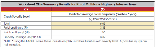
STEP 2: Following input in Step 1, the spreadsheet tools automatically calculated the predicted number of crashes. To review example results for the intersection calculations, see the CMF results for Alternative #1 (shown in Worksheet 2B) and predicted number of crashes (Worksheet 2C):
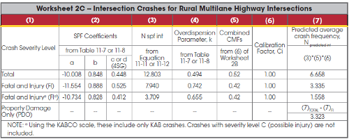
Summary results are shown in Worksheet 2E. The intersection analysis results for Alternative #1 are shown below. The shaded region identifies the summary data used in Step 3.
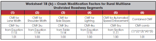
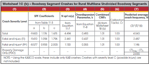
Similarly, the Alternative #1 spreadsheet results for segment calculations (Worksheets 1B, 1C, and 1E) are shown as:
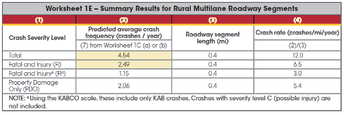
STEP 3: Summarize the total number of crashes.
This activity can be performed manually or summarized on the "Rural Multilane Site Total" sheet (note that the analyst will need to customize this table to link to individual worksheets as needed). The Alternative #2 results are also depicted in the table. The results are summarized as follows:
| Alternative | Total Crashes per Year | FI Crashes per Year | ||||
|---|---|---|---|---|---|---|
| Intersection Crashes | Segment Crashes | Predicted Crashes | Intersection Crashes | Segment Crashes | Predicted Crashes | |
| Existing | 12.8 | 4.34 | 17.14 (say 18) |
7.94 | 2.37 | 10.31 (say 11) |
| Alternative #1 | 6.66 | 4.54 | 11.2 (say 12) |
3.33 | 2.49 | 5.82 (say 6) |
| Alternative #2 | 6.66 | 4.68 | 11.33 (say 12) |
3.33 | 2.56 | 5.89 (say 6) |
| Comparison of Existing and Alternative #1 Predicted Crash Reductions | ||||||
| Difference | 12.80 – 6.66 = 6.14 | 4.34 – 4.54 = -0.2 | 17.14 – 11.20 =5.94 (say 6) | 7.94 – 3.33 = 4.61 | 2.37 – 2.49= -0.12 | 10.31 – 5.82 = 4.49 (say 5) |
| Percent Reduction | 48.00% | -4.60% | 35% | 58.10% | -5.06% | 43% |
| Comparison of Existing and Alternative #2 Predicted Crash Reductions | ||||||
| Difference | 12.80 – 6.66 = 6.14 | 4.34 – 4.68 = -0.34 | 17.14 – 11.33 =5.81 (say 6) | 7.94 – 3.33 = 4.61 | 2.37 – 2.56 = -0.19 | 10.31 – 5.89 = 4.42 (say 5) |
| Percent Reduction | 48.00% | -7.80% | 35% | 58.10% | -8.02% | 43% |
Note: FI = fatality and injury
The spreadsheet values do not include any rounding errors as would be expected when performing hand calculations. As a result, these numbers should be similar but may not exactly match predicted crashes calculated manually.
Based solely on an evaluation of the predicted number of crashes, a road with the characteristics described for the existing design configuration can be expected to experience approximately 18 crashes per year, of which about 11 would involve an injury. For locations where a left-turn lane is added with standard-use lanes of 11-ft. wide and shoulder widths of 6-ft. wide (Alternative #1), the total number of predicted crashes per year reduces to approximately 12 with 6 involving an injury. In contrast, an approach with a left-turn lane, standard-use lane widths of 12-ft., but shoulder widths of 4-ft. (Alternative #2) similarly results in 12 predicted crashes with 6 involving an injury.
For the conditions outlined in this problem, the addition of a left-turn lane provides added value as it can be expected to result in a reduction of approximately 35 percent in the total number of crashes and approximately a 43 percent reduction in FI crashes. The two alternatives considered provide very similar results, and so the analyst can conclude that either Alternative #1 or Alternative #2, if constructed, will result in the predicted crash reductions.
These calculations are based only on predicted crash performance, but do not consider potential operational issues. For example, vehicles positioned in the narrow 10-ft. left-turn lane as shown for both alternatives may encroach on the adjacent travel lane.
While this example focused on left-turn lane options, it is advisable for an analyst to conduct similar safety assessments for right-turn treatments.
The HSM procedures require the analyst to understand how the SPFs and CMFs equate to the base conditions associated with the procedure. Incorrect use of these values can introduce erroneous results. This example compared the crash predictions, and so the use of a calibration factor with a value of 1.0 can be used for comparison purposes. If the analyst would like to record findings as crash frequency instead of percent reduction in the number of crashes, calibrated SPFs with known calibration factors should be used for the analysis. A more detailed analysis during the design phase would provide additional useful information about predicted crashes.
A common method for evaluating design alternatives is to use CMF comparisons that do not directly consider traffic volume. This approach is less reliable than the predictive methods, but can be used to evaluate alternatives when an SPF is not available for the condition or when a simple comparison between two alternatives is all that is needed.
If the project progresses to the design stage, and should the historical (observed) crash data become available at that time, the analyst could use the advanced safety assessment method to further evaluate existing conditions and future designs with minor changes. Future configurations that include major changes are not suitable for the SPF with CMF Weighted with Observed Crashes method as the observed crashes would no longer be representative of the new configuration.
![]()
Note: See table 3 for a full definition of Project Type designations. Source: This example problem is based on a case study for Arizona SR 264 Burnside Junction to Summit posted at https://www.fhwa.dot.gov/design/pbpd/case_studies.cfm.
As part of a 34.5-mile long, two-lane rural highway reconstruction project to enhance a developing freight route, a transportation agency would like to evaluate the estimated safety implications of two alternative designs. The current two-lane rural highway has intermittent right– and left-turning lanes and infrequent passing lanes. The existing horizontal and vertical geometry information has been acquired using a survey and was confirmed against the original as—built plans. As part of the project, the transportation agency has included the geometric information into a civil design software package. The two alternatives currently under consideration are defined as Alternative A and Alternative B.
Alternative A – Widen Existing Roadway to 34-ft.
The purpose of Alternative A is to widen the existing roadway to 34-ft. to provide 5-ft. shoulders by widening the existing 1-ft. shoulders to 5-ft. shoulders. The existing travel lane width would remain 12 ft. The improvements would include adding center line and shoulder rumble strips, flattening side slopes, installing guardrail, extending drainage structures, and providing delineators and recessed pavement markers.
Alternative B – Widen Existing Roadway to 40-ft.
The purpose of Alternative B is to widen the existing roadway to 40-ft. to provide full-width shoulders. The proposed improvements would widen the existing 1-ft. shoulders to 8-ft. shoulders. The existing travel lane width would remain 12-ft. The improvements would include adding center line and shoulder rumble strips, flattening side slopes, installing guardrail, extending drainage structures, and providing delineators and recessed pavement markers.
The Project Type is 3R and the Related Task is Alternative Selection. How can the analyst estimate the difference in the average annual crash reduction for a 5-ft. shoulder compared to that of an 8-ft. shoulder over a 20-year period?The 2010 AADT, 4-year crash counts, and the manner of collision are provided in the following tables. The first table also shows projected AADT values for the design year 2036.
AADT(vpd)
| Mile Post (MP) | 2010 AADT | 2036 Projected AADT |
|---|---|---|
| MP 441.02-MP 446.18 | 5,010 | 9,900 |
| MP 446.18-MP 446.91 | 6,429 | 12,150 |
| MP 446.91-MP 448.37 | 5,199 | 7,350 |
| MP 448.37-MP 475.50 | 4,102 | 5,400 |
Note: AADT = average annual daily traffic, vpd = vehicles per day
| Crash Severity | Number of Crashes |
|---|---|
| Fatal | 6 |
| Incapacitating Injury | 3 |
| Non-Incapacitating Injury | 1 |
| Possible Injury | 24 |
| No Injury (PDO) | 22 |
| Total Crashes | 56 |
Note: PDO = property damage only
| Crash Severity | Number of Crashes |
|---|---|
| Head On | 2 |
| Left Turn | 3 |
| Rear End | 13 |
| Angle (Other than Left Turn) | 5 |
| Sideswipe (Opposite Direction) | 2 |
| Sideswipe (Same Direction) | 4 |
| Single Vehicle | 27 |
| Total Crashes | 56 |
The following table shows the road characteristics for the various configurations. For informational purposes, the table shows the base conditions associated with a rural two-lane highway in the HSM. Notable variations from the base conditions include the shoulder width, roadside hazard rating, and center line rumble strips.
Road Characteristics (Existing and Proposed) for the Rural Two-Lane, Two Way Road
| Roadway Element | Existing | Alternative A | Alternative B | HSM Base Condition |
|---|---|---|---|---|
| Lane width (ft) | 12 | 12 | 12 | 12 |
| Shoulder width (ft) | 1 | 5 | 8 | 6 |
| Shoulder type | Paved | Paved | Paved | Paved |
| Roadside hazard rating | Varies (6 or 7 most frequent) | Varies (1 or 2 most frequent) | Varies (1 or 2 most frequent) | 3 |
| Driveway Density | Per survey | Per survey | Per survey | ≤ 5 per mile |
| Horizontal curves: length, radius, and presence or absence of spiral transitions | Per best fit alignment | Per best fit alignment (match existing) | Per best fit alignment (match existing) | None |
| Horizontal curves: Superelevation | Per as-builts & survey | Per as-builts & survey (match existing) | Per as-builts & survey (match existing) | None |
| Grades | Per as-builts & survey | Per as-builts & survey (match existing) | Per as-builts & survey (match existing) | None |
| Center line rumble strips | None | Present | Present | None |
| Passing lanes | Per survey | Per survey (match existing) | Per survey (match existing) | None |
| Two-way left-turn lanes | Per survey | Per survey (match existing) | Per survey (match existing) | None |
| Lighting | Present at Intersection | Present at Intersection (match existing) | Present at Intersection (match existing) | None |
| Automated speed enforcement | None | None | None | None |
HSM = Highway Safety Manual.
The analyst can first inspect Table 8 to identify potential safety assessment methods for a 3R project type and the alternative selection task (see Table 3 for a full definition of the 3R project type). Five potential methods (two basic, two intermediate, and one advanced) may be considered for this analysis. Because the alternatives require comparisons of varying geometric characteristics, an assessment method that includes CMFs is appropriate (thus eliminating the AADT-Only SPF). The study corridor is lengthy (almost 35 miles long) and the traffic volume and road characteristics vary throughout the corridor. Because the analyst would like to verify that the increase in traffic volume is considered in the analysis, the two basic methods are eliminated from consideration.
The remaining two potential safety assessment methods use procedures specific to the HSM. The SPF with CMF Adjustment can be used to evaluate the predicted number of crashes along a corridor with similar characteristics to the study site. The SPF with CMF Weighted with Observed Crashes includes the crash history so that the safety assessment includes consideration of the recent crash history at the location. Both of these safety assessment methods can be used.
To help select the method, the analyst reviews the length of the corridor and the varying road characteristic information and notes that the alignment information is already included in a civil design software package. The proposed analysis is impractical to conduct using hand calculations. Both of the methods can be performed, however, using the HSM "Smart Spreadsheets" and the FHWA IHSDM analysis software. The IHSDM has an added benefit in that it can directly import road characteristic data from a civil design software program with little to no additional manual entry. The selection of IHSDM, therefore, will enable the use of an advanced safety assessment method while also streamlining the analysis process. The web address to acquire this free software tool is provided in the "Detailed Analysis" section of this problem.
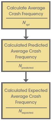
The HSM can be used to estimate the number of predicted crashes for a rural, two-lane highway by applying the procedures introduced in HSM Chapter 10 (pp. 10-1 to 10-74). By determining predicted crashes, the analyst can estimate how many crashes may be expected for a specific road type with varying road conditions (in this case the curve radii and traffic volumes). Once the predicted number of crashes is known, the expected number of crashes for a specific site can be calculated by applying the Empirical Bayes Method summarized in HSM, Part C (Volume 2), pp. A-15 to A-23.
The IHSDM analysis software can be used to calculate the expected average crash counts for the existing conditions and the given alternatives for the 20-year study period. If a State has calibrated the SPF contained in the HSM or has developed its own SPF that has a similar equation format (functional form) as the HSM equation, these values can be directly inserted into the IHSDM.
To calculate the expected average crash frequency for the existing conditions and the proposed alternatives, download the IHSDM analysis software. This product can be downloaded free of charge at http://www.ihsdm.org. Two training courses are available through the Federal Highway Administration's National Highway Institute for those that would like to learn more about how to use the software (http://www.nhi.fhwa.dot.gov/training/course_search.aspx?tab=0&key=IHSDM&res=1).
STEP 1: Input (or import) the vertical and horizontal roadway alignments into IHSDM.
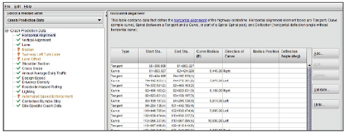
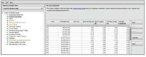
The following figures are screen shots of what the alignments should look like following input into IHSDM.
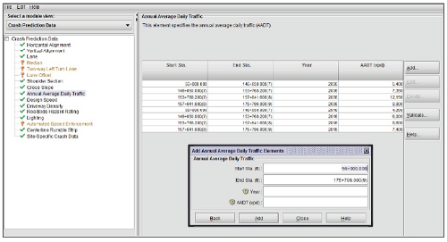
STEP 2: Input all remaining crash prediction data for the existing conditions.
Like the alignment data, all other data is entered using the roadway stationing. The following figure shows what the input data for AADT looks like.
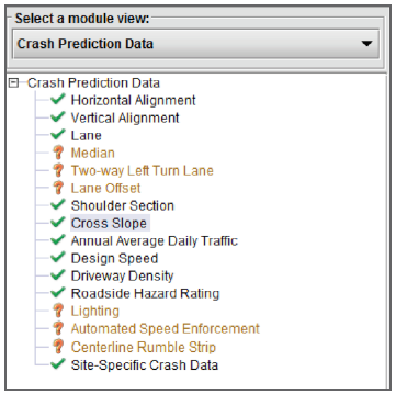
The following figure shows all data that must be entered before running the Crash Prediction Module. Items with a green check show that required data was entered. An orange question mark represents data for which default values are being used because the analyst did not provide site specific information. A red "X" will appear by the data set if the required data is missing. This process of creating or importing a new highway must be followed for each alternative.
STEP 3: Run the crash prediction analysis within IHSDM.
IHSDM has the ability to create a summary, report, raw results, graphs, and spreadsheets of the analysis. The following table shows a summary of the results for expected crashes based on output from the IHSDM software analysis.
2016-2036 Expected Total Number of Crashes
| Crash Severity Levels | Existing Conditions 1-ft. Shoulder | Alternative A 5-ft. Shoulders | Alternative B 8-ft. Shoulders |
|---|---|---|---|
| Total | 636.38 | 531.58 | 504.16 |
| Fatal and Injury | 283.40 | 230.45 | 216.80 |
| Property Damage Only | 352.98 | 301.13 | 287.36 |
| Reduction in Total Crashes | NA | 104.80 (say 105) | 132.22 (say 133) |
2016-2036 Expected Average Annual Crash Frequency
| Crash Severity Levels | Existing Conditions 1-ft. Shoulder | Alternative A 5-ft. Shoulders | Alternative B 8-ft. Shoulders |
|---|---|---|---|
| Total | 31.82 | 26.58 | 25.21 |
| Fatal and Injury | 14.17 | 11.52 | 10.84 |
| Property Damage Only | 17.65 | 15.05 | 14.37 |
| Reduction in Total Crashes | NA | 5.24 (say 6) | 6.61 (say 7) |
The proposed improvements for alternatives A and B respectively reduce the expected number of crashes compared to the existing conditions by 105 and 133 crashes, respectively, projected over a 20-year period. Alternatives A and B have an annual average crash reduction of 6 and 7 crashes per year, respectively. Based on the predictive method analysis, Alternative B, with the 8-ft. shoulder, will have an average annual reduction of between one and two more crashes per year than Alternative A, with a 5-ft. shoulder. This information on safety performance could then be considered alongside other project criteria.
The analyst should confirm that data is entered (or imported) and used correctly in the IHDSM analysis software. IHSDM only takes into account those SPFs and CMFs associated with the HSM or that have been input (as previously indicated). The HSM procedures and the IHSDM are updated periodically with the most recent safety knowledge. Before starting an analysis, it is a good idea to confirm that you are always using the most recent version of the IHSDM software. As noted in the "Detailed Analysis" section of this problem, the IHSDM software and information about using the software can be found at the web address http://www.ihsdm.org.
The expectation to include traffic volume as well as changes in road characteristics narrowed down the suitable analysis tools to those that used SPFs with CMFs. This analysis could also have used the HSM spreadsheets presented in Problem 3.2. In addition, the findings from this analysis can be used as input into an economic appraisal such as a benefit/cost ratio or prioritization method such as incremental benefit/cost ratio.
![]()
Note: See table 3 for a full definition of Project Type designations.
A State DOT is examining a 0.5-mile long urban freeway connector (loop) ramp to evaluate whether changes are needed for possible removal, improvement, or replacement due to recurring congestion. As part of this analysis, the DOT is conducting a safety assessment to determine whether the loop ramp has more crashes than would be expected for similar ramps. The Project Type is 4R and the Related Task is to document analysis for a potential Interchange Justification Request. How can the analyst predict the estimated number of crashes for this interchange freeway loop ramp for a 3-year study period between 2013 and 2015 while directly considering the AADT in the analysis?
In 2013, the ramp had an AADT of 9,800 vpd. Other ramp characteristics are summarized as follows:
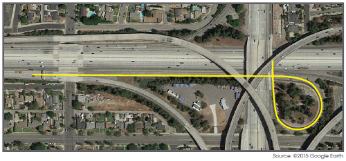
The following aerial photograph depicts the ramp configuration (center line highlighted with yellow).
Crash data for the corridor during the study period is summarized in the following table. The small number of observed crashes at this location provides information about observed crash frequency. For this example, the observed crash information is available for estimating future safety performance. The small crash frequencies observed would not be useful for identifying prospective countermeasures.
| Year | Property Damage Only Crashes | Fatal and Injury Crashes | ||
|---|---|---|---|---|
| Multiple vehicles | Single-vehicle | Multiple vehicles | Single-vehicle | |
| 2013 | 0 | 1 | 0 | 1 |
| 2014 | 1 | 0 | 0 | 0 |
| 2015 | 0 | 1 | 0 | 0 |
The analyst can evaluate the candidate safety assessment methods shown in Table 8. The Interchange Justification Request task and the 4R project type are associated with five potential safety assessment methods: two basic, two intermediate, and one advanced. Because the goal is to comprehensively assess the varying ramp geometric features and calculate the estimated number of crashes, an assessment method that includes CMFs is appropriate (thus eliminating the AADT-Only SPF). The analyst would like to verify the influence of traffic volume over the three-year study period. This requires a volume-based approach (i.e. methods that use an SPF). The two basic methods should therefore be eliminated from consideration as they do not include traffic volume in the analysis.
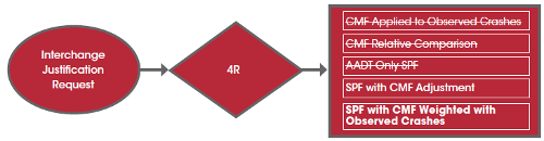
The remaining two potential safety assessment methods use procedures specific to the HSM. The SPF with CMF Adjustment can be used to evaluate the predicted number of crashes along a corridor with similar characteristics to the study site. The SPF with CMF Weighted with Observed Crashes includes the crash history so that the safety assessment includes consideration of the recent crash history at the location. Both of these safety assessment methods can be used, but the site-specific emphasis provides additional confidence that the calculated numbers reflect the expected number of crashes for the specific study site. For this reason, the analyst selects the SPF with CMF Weighted with Observed Crashes method.
The analyst has the following three available options for performing the analysis for this method:
The choice between the two automated tools is simply a preference issue as they both correspond to the HSM approach for this analysis. For this assessment, the analyst selected ISATe. The web address to acquire this free software tool is provided in the "Detailed Analysis" section of this problem.
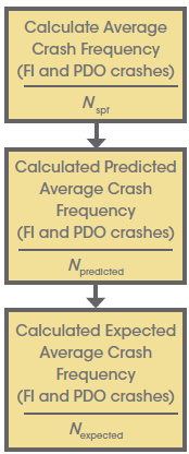
The 2014 HSM Supplement can be used to estimate the number of expected crashes for a freeway or a ramp. The procedure for ramps is introduced in SM Chapter 19 (pp. 19-1 to 19-152). By determining predicted crashes, the analyst can estimate how many crashes may be estimated for a specific ramp with varying road conditions (in this case multiple horizontal curves and varying barrier to the right and left). Once the predicted number of crashes is known, the expected number of crashes for a specific site can be calculated by applying the Empirical Bayes Method summarized in the 2014 HSM Supplement, pp. B-14 to B-30.
As previously indicated, the analyst has selected the advanced method for an SPF with CMF Weighted with Observed Crashes. This assessment is for a specific location with a known crash history and so the procedure calculates the expected number of crashes. Because the ramp's cross-sectional characteristics are consistent along its entire length, the ramp can be modeled as one segment.
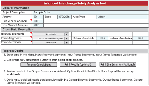
To calculate the expected average crash frequency for the existing ramp location, the analyst has decided to use ISATe, a free software self-calculating spreadsheet tool. This product can be downloaded free of charge at http://www.highwaysafetymanual.org/Pages/tools_sub.aspx. The following steps summarize the process for performing the calculations to evaluate the expected crashes.
STEP 1: Enter known data.
The analyst enters the geometry, traffic, and crash data into the ISATe program. The analysis is conducted by automating the calculations using the program and reviewing the results. ISATe provides the analyst with expected crash frequencies for the ramp and also outputs CMF values to help the analyst identify roadway characteristics that could be changed to reduce crash frequency.
STEP 2: Divide the ramp into homogeneous segments.
The beginning and ending of the ramp are defined as the gore nose where the ramp joins each freeway mainline. This particular ramp does not need to be divided into segments because its cross-sectional characteristics are consistent throughout its length, and ISATe can model a ramp with up to five horizontal curves along its length.
STEP 3: Specify analysis period, analysis type, and area type in the ISATe "Main" worksheet.
For this analysis, the time period of interest is defined as the years 2013-2015. Crash data are available, so the empirical Bayes analysis procedure that is built into ISATe will be used. The area type is specified as urban.
STEP 4: Enter input data into the ISATe "Input Ramp Segments" worksheet.
This worksheet contains two columns to describe each ramp segment (for the crash period and the study period) and rows for each input data element. In this example problem, the crash period and the study period are the same time period, and no potential modifications to this ramp are being considered, so the input data for the crash period and the study period are the same. For some analyses (e.g., if a projection of future crash counts is desired), a study period in the future can be specified, while the crash period always must be in the past.
As shown in the aerial photo, the loop ramp is a single-lane ramp with two horizontal curves. The first curve is gradual (radius = 11,460 ft) and is located under the freeway mainline bridge. The second curve is sharp (radius = 150 ft) and is located in the southeast quadrant of the interchange.
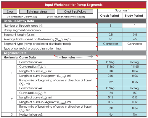
Cross section data and roadside data are entered as shown. The analyst should input specific information for a total of five barrier sections – three located on the left side of the ramp (in the direction of travel) and two located on the right side of the ramp.
The analyst should next enter ramp access and traffic data. These data include the presence and lengths of ramp entrances or exits on each segment, and presence of weaving sections. The analyst provides traffic volumes for the years 2013, and ISATe uses the same traffic volume for the years 2014 and 2015.
Crash data are entered and broken down by crash type, severity, and year.
Once all input data are entered into the "Input Ramp Segments" worksheet, the analyst should click the "Check Input Values" button to verify that no illogical or erroneous data values were entered.
STEP 5: Perform the analysis calculations.
The analyst clicks the "Perform Calculations" button on the "Main" worksheet of ISATe to initiate calculations.
STEP 6: Review the calculation results.
ISATe provides a summary of the calculation results on the "Output Summary" worksheet. In this example problem, the freeway facility of interest consists of one ramp segment. ISATe can also be used to analyze a facility that consists of a combination of mainline segments, ramp segments, and crossroad ramp terminals.
For the entire analysis period (2013-2015), the ramp is expected to experience about nine crashes, of which about six will be PDO. These values are equivalent to expected crash frequencies of about three crashes per year, of which about two will be PDO.
By using the ISATe spreadsheet program to evaluate the loop ramp, the analyst estimates that the expected crash frequency is about three crashes per year. Over the entire analysis period, this equates to about nine crashes. These computed numbers are consistent with the observed crash counts. The analyst can conduct similar analyses on other loop ramps and compare the values for this location to assess whether they are notably higher than those for similar locations.
It is possible for the analyst to enter erroneous input data or to enter values that are illogical when compared across several input elements. For example, a roadside barrier lateral offset cannot be located closer to the travel lane than the width of the shoulder. The ISATe program contains many data validation mechanisms to minimize this possibility, and a checking feature is also available by clicking the "Check Input Values" button on the input data worksheets.
This analysis can also be performed by hand-calculating the ramp safety prediction methodology described in Chapter 19 of the HSM (see Appendix item A-3.4). Due to the extensive nature of the calculations, however, the hand-calculated method is time consuming and can be cumbersome due to the large number of equations included in the methodology.
The FHWA software tool IHSDM, however, could also be used to conduct this analysis. The crash module for the IHSDM includes a "site-based analysis tool" that can be used without having to include the detailed horizontal and vertical alignment and cross-section data noted in Example Problem 3.3. The selection of ISATe versus IHSDM is a matter of personal preference since both of these free tools perform the same analysis. The IHSDM software is available for download at http://www.ihsdm.org.

