U.S. Department of Transportation
Federal Highway Administration
1200 New Jersey Avenue, SE
Washington, DC 20590
202-366-4000
| < Previous | Table of Contents | Next > |
Step 6 in the scalable risk assessment process is to use the analytic method selected in Step 5 to estimate the desired exposure measure(s). All of the previous steps involve making scoping or planning decisions about how to estimate exposure. Step 6 in the process is when the detailed analysis for exposure estimation occurs, As a result, the Step 6 section in this guide is the largest and has the most content.
Step 6 includes a section for each of the three primary methods that can be used to estimate exposure.
Site counts are direct measurements of the number of pedestrians or bicyclists at a defined location. The counts may be gathered automatically from various technology-based sensors or manually from human observers. Site counts are taken at a point and are typically used to represent two different scales: point and segmentFor the point scale, counts are most commonly used for intersection crosswalks. For the segment scale, the site count (taken at a point) is applied to the entire length of a street segment (where the counts are not expected to vary significantly along the segment length),
Counts are more commonly used to estimate exposure when the desired facility coverage is limited, as count data collection for all facilities within a large network or region is cost-prohibitive (unless extensive sampling is used)In some cases, it is also a challenge to get representative pedestrian and bicyclist counts due to seasonal and day-of-week variation.
This section of Step 6 provides an overview of counting procedures for pedestrians and bicyclistsIn particular, this section will highlight considerations and issues that are relevant to site counts used for exposure estimation. Analysts will find many more procedural details in the comprehensive guidance documents listed in Table 15.
| Guidance Document or Report | Useful Resources or Application |
|---|---|
| FHWA 2016 Traffic Monitoring Guide, Chapter 4 Traffic Monitoring for Non-Motorized Traffic |
|
| Report FHWA-HEP-17-011, Coding Nonmotorized Station Location Information in the 2016 Traffic Monitoring Guide Format, 2016 |
|
| Report FHWA-HEP-17-012, FHWA Bicycle-Pedestrian Count Technology Pilot Project - Summary Report, 2016 |
|
| NCHRP Report 797, Guidebook on Pedestrian and Bicycle Volume Data Collection, 2014 |
|
| NCHRP Web-Only Document 229, Methods and Technologies for Pedestrian and Bicycle Data Collection: Phase 2, 2016 |
|
| Report FHWA-HPL-16-026, Exploring Pedestrian Counting Procedures: A Review and Compilation of Existing Procedures, Good Practices, and Recommendations, May 2016 |
|
| Alta Planning + Design, Innovation in Bicycle and Pedestrian Counts: A Review of Emerging Technology, 2016 |
|
In some exposure analyses, site counts may serve as the only source of data for exposure estimationHowever, the collection of site counts on all street segments or at all signalized intersections within a city or region is cost-prohibitive. Therefore, the use of site counts only is most applicable to exposure analyses that are facility-specific (i.e., point or segment scale) and focus on a limited number of intersections or street segments.
In most exposure analyses, site counts are collected at a small but representative sample of locations, and then an estimation model is developed and calibrated from these site counts and used to estimate pedestrian and bicyclist volumes at uncounted locations. The next major section in this chapter describes several different demand estimation models that use a sample of site counts and other street inventory and land use variables to predict pedestrian and bicyclist volumes at all locations citywide.
Some cities, MPOs, and state DOTs have begun to collect pedestrian and bicyclist counts as part of a routine monitoring program, so it may not be necessary to start from the beginning for exposure estimationOne should inquire about existing count data not just with transportation agencies, but also with other groups and agencies that may share your interest in pedestrian and bicyclist activity:
Even if other agencies' existing counts can be used, it is likely that additional counts will be desired for the purposes of exposure estimationIn some cities, the existing and ongoing counts are at a very limited number of locations, and may have been chosen because of high pedestrian and bicyclist usage or recent facility improvements. For purposes of exposure estimation, additional counts may be needed at high crash locations or at a broader range of locations that represent a mix of facility types and land uses (for purposes of estimation model development and calibration).
Site counts can be conducted for varying durations (e.g., 12 hours, 48 hours, 7 days, etc.) and at different times of the year, but the final count measure most commonly used in both motorized and non-motorized exposure estimation is AADT. In these cases, AADT is applied to a defined segment, and is then multiplied by the defined segment length to calculate average annual daily PMT or BMTThe same process can be used at intersection crossings, whereby the crossing length is used to calculate PMT or BMT at each crossingEarlier in this guide, Step 4 described a simple example of this calculation process.
The estimation of AADT from a short duration site count is a recommended practice for pedestrian and bicyclist exposure estimation. AADT estimates are typically made using what are called factor adjustments (described in detail in Section 4.4 of FHWA's Traffic Monitoring Guide). Aside from being a widely accepted practice in motor vehicle analysis, there are several reasons why AADT values should be estimated and used in exposure analysis. Pedestrian and bicyclist counts can vary dramatically by month of the year, day of the week, and by prevailing weather conditionsSite counts that were collected for a single day during favorable weather are not a representative sample of all other days during the year. Therefore, in simple terms, the factor adjustment process is used to adjust the count samples to represent more accurately the true annual average pedestrian and bicyclist usage.
The factor adjustment process for AADT estimation requires continuous count data from similar location(s) to scale accurately a short duration count to represent an annual average countHowever, some cities or regions may not have the required continuous count data for factor adjustment. At the time of this Guide development, many agencies are still working to implement the factor adjustment processSeveral organizations are currently working to develop default seasonal adjustment factors based on climate zones.1 If factor adjustment and AADT estimation is not feasible for your application, every effort should be made to collect site counts during seasons/months, days of the week, and weather conditions that most closely resemble typical conditions during the year.
The following paragraphs describe key considerations when collecting counts specifically for exposure estimation. Many of these considerations are addressed in more detail in other data collection guides, but are highlighted here to emphasize their importance.
Use automated counter equipment as much as possible: Automated counter equipment allows counts to be conducted for longer periods (multiple days), which reduces error in AADT estimates. Automated counter equipment can also reduce the labor cost of data collection. The resources listed at the beginning of this Site Counts section provide detailed guidance on selecting the appropriate technologies for automated counting.
Avoid very short duration counts (i.e., two-hour counts): The FHWA Traffic Monitoring Guide recommends a minimum duration of seven days for short duration countsIf this duration is not cost-feasible at all of the desired locations, then at least one to two twelve-hour periods should be counted. Two-hour counts should be avoided as much as possible, even it if means reducing the number of count locations to allow for a six-hour or twelve-hour countSeveral research efforts have documented the high error rates that result from estimating AADT from two-hour counts.
Seek balance between number of count locations and duration: As implied in the previous bullet, it may be necessary to balance the number of count locations with the duration of each count. This may be necessary to avoid very short duration counts yet still collect data at a representative number of count locationsIn these cases, one is balancing the temporal error (from sampling short durations of time during the year) with the spatial error (from sampling very few locations of all locations to be analyzed). At this time, achieving a balance between number of count locations and count duration is considered more of an art form and not science.
Select representative months and days of week for your area and count location: Site counts should be collected during typical or normal seasons/days/times, especially if adjustment factors are not feasible to use for estimating AADT valuesEven if adjustment factors are planned for use, site counts should be collected during months/days/times that are considered typical or normal conditionsThis helps to reduce the magnitude of the factor adjustment, and ultimately, reduce the error associated with AADT estimates.
Focus on balance of high-priority yet representative locations: If site counts must be collected specifically for exposure estimation, the count collection effort should focus on a balance of high-priority yet representative locations. High priority locations for exposure analysis are likely to be those locations that have a high crash frequency. However, if an estimation model is to be developed, site counts at high-crash locations are likely to be a biased input for model developmentThe result is an estimation model that only predicts counts accurately at high-crash locations. Therefore, high-crash locations should be balanced with other locations that represent a range of facility types and land use patterns. Note that this balance is considered a more of an art form and not science at this time.
As described in Step 5, there are several estimation models to estimate pedestrian and bicyclist demand for input to an exposure measureIn this section of Step 6, we provide a detailed overview and key considerations in developing direct demand models since they are the most widely used tools in the literature for pedestrian and bicyclist volume estimation modeling. Specifically, detailed overview of direct demand models is presented first, and then step-by-step instructions are provided (with examples) to develop a direct demand model.
Direct demand models are the most widely used tools in the literature for pedestrian and bicyclist volume estimation modeling (especially in supporting traffic safety studies). These models have been primarily used to develop facility-specific demand estimations for the local level of community, project, and facility planning and to evaluate and prioritize projects. The potential usages of direct demand models are listed as follows by Kuzmyak et. al.l (2014):
The FHWA has sponsored a Non-Motorized Travel Analysis Toolkit, which includes various applications to support non-motorized transportation planning and modeling. This Toolkit includes several direct demand models to estimate pedestrian and bicycle volumes (http://www.nmtk.pedbikeinfo.org/ui/#/). Direct demand models have also been identified as the primary tools to measure bicyclist and pedestrian exposure for safety analysis.
Direct demand models are generally based on different versions of regression modeling to explain “demand levels as recorded in counts as a function of measured characteristics of the adjacent environment” (Kuzmyak et. al. 2014). As indicated by Munira and Sener (2017), “the concept of using a direct-demand model to estimate non-motorized activity is not newStudies dating back 50 years have forecast non-motorized traffic using count and spatial data.” Schmiedeskamp and Zhao (2016) explained such models as following “a similar approach of first proposing a set of explanatory variables, fitting some form of regression model, and then interpreting and justifying the results according to the guiding theory.” Direct demand models are based on variety of data sources such as activity counts, census population and employment characteristics, land use and topography and transportation network characteristics.
Direct demand models are appealing due to their simplicity and convenience in development and application, and since they are generally based on available dataThese models are particularly useful for screening and preliminary analyses especially when the resources are limited and a more comprehensive (and relatively expensive) model is not available or not possible to developHowever, direct demand models are limited in terms of capturing the behavioral structureIn addition, they are usually not transferable due to their strong linkage to local context, activity levels and the characteristics that the models are built on Aoun et. a. l(2015) summarized the advantages and disadvantages of direct demand models as in Table 16.
| Advantages | Disadvantages |
|---|---|
|
|
Source: (adapted from) Aoun et. al. 2015
Kuzmyak et. al. (2014) highlighted the need to be judicious in the development and application of direct demand models, and suggested the following guidelines:
The readers are referred to Munira and Sener (2017) for an in-depth review of the available literature associated with direct-demand modeling to estimate bicycle and pedestrian activity.
This section provides step-by-step instructions to develop a direct demand model.
The generalized approach to develop a direct demand model includes three primary phases as demonstrated in Figure 17

Figure 17. Direct Demand Model Development Process
In addition, Figure 18 provides a flowchart of an algorithm to help the analysts walk through the tasks needed to complete the phases when developing a direct demand model
Below, we provide detailed instructions on each phase, and the corresponding tasks involved in each phase as consistent with the flowchart provided in Figure 18Specifically, the main objective and primary tasks of each phase are presented first, followed by discussion of key considerations when processing the phase.
![This map and text graphic shows locations in Seattle that have high pedestrian risk, based on the measure of expected pedestrian crashesText graphic: 'Systematic vsHigh Crash Approach to Reducing CrashesA systematic approach 1) proactively identifies sites based on risk factors associated with a particular crash type, and 2) uses cost-effective strategies to address potential safety issues system-wideThese strategies might include locations with and without a crash history This allows us to address future safety risks before they become an issues This approach complements our traditional high-collision analysis, which identifies and recommends safety improvements for locations with a high number of crashes ['hot spots'] We'll also continue to address safety concerns at bicycle or pedestrian crash 'hot spot' locations.](images/fig18_lg.jpg)
Figure 18. Direct Demand Model Development Detailed Flow Chart
Objective: The main objective of Phase A is to identify the study focus.
Primary Tasks: Phase A includes three primary tasks:
Processing the Phase:
Task 1: Phase A starts with identification of the overall study area (or target population) for which the direct demand model is desired to be developedWhen executing the task, it is of utmost importance to identify project objectives to avoid any unnecessary process, optimize the limited resources and limit the bias.
Task 2: The next task is to determine the facility locations at which the exposure measure is desiredExample of facility locations include signalized and unsignalized intersections or midblock locations along the street segmentsStep 3 of this Guide provides information on how to determine desired geographic scale(s) for exposure.
Task 3: Once the location-specific details of the model are identified, the analyst needs to determine the variable of interest, i.ethe model output or outcome whose variation is being examinedFor example, in the context of non-motorized direct demand models, the analyst might be interested in obtaining annual average pedestrian volume and peak hour bicycle traffic volumeIn statistical terms, the variable of interest is named as the dependent variable of the model.
Objective: The main objective of Phase B is to prepare the data needed for model development.
Primary Tasks: Phase B includes five primary tasks:
Processing the Phase:
Task 1: The first task in this phase is to compile data needed for the dependent variable of the modelAs aforementioned in the Site Counts part of Step 6 of this Guide, site counts serve as the common source of data for exposure estimation especially when the desired facility coverage is limited and data collection for all facilities within a large network or region is cost-prohibitiveTherefore, site counts are the main ingredient used for creating the dependent variable of the model
Sampling: In the ideal conditions, it is desired to have site counts at all facility locations across the study area, but this is not feasible given the limited amount of resources (i.ebudget, time, equipment and manpower constraints)Therefore, the analyst needs to develop a sampling strategy to select sites from which data will be collectedThere are two different types of sampling technique for data collection: non-probabilistic sampling technique and probabilistic sampling technique
Non-probabilistic sampling techniques are the most commonly used techniques due to their low cost, easy-to-implement methodologyIn this technique, the analyst identifies some subjective criteria (e.gconvenience, engineering judgment, local knowledge, quota, etc.) and collects data based on those criteriaThis technique does not allow the analyst to control for sampling error, and usually a small number of samples are collectedIf the analyst needs to draw conclusions about the entire population, this technique is not recommended since the sites collected might not be representative.
Probabilistic sampling techniques are based on statistical approaches, involves random selection process, and therefore allows the analyst to compute a sample size and to draw conclusions about the entire populationIn general, this technique requires more resources because of the increased sample size needed to obtain a representative sampleThere are various different methodologies that can be selected in applying probabilistic sampling techniques including simple random sampling, strategic sampling, cluster analysis and multi-stage random sampling.
Table 17 is adapted from Greene-Roesel et. al. 2010 and provides summary information on each of these sampling techniques
| Sampling Technique | Methodology | Definition | Example | Advantage | Disadvantage |
|---|---|---|---|---|---|
| Non-probabilistic method | Convenience | Obtaining a sample of people or units that are most convenient to study | Selecting intersections with available collision data | Low Cost; Easy method of sample design | No representative sample; Not recommended for descriptive or casual studies |
| Judgement | Selecting a sample based on individual judgment about the desirable characteristics required of the sampling units. | Selecting signalized intersections because of experience or intuition that they have higher pedestrian flow. | Low cost; Allow to draw some conclusions about the characteristics of the selected sample. | Does not allow drawing general conclusions about the entire population. | |
| Quota | It is similar to the judgment sample, but requires that the various subgroups in a population are represented. | Making sure to select some signalized and some unsignalized intersections in a sample. | Low cost; Allow to draw some conclusions about the characteristics of the selected sample. | Does not allow drawing general conclusions about the entire population, or sample subgroups. | |
| Snowball | Additional survey respondents are obtained from information provided by the initial sample of respondents. | Used when surveying individuals about their behaviors (e.ghow much they walk in specific areas) | Some characteristics about the target population can be known | Requires a lot of time and resources; Used only for surveys. | |
| Probabilistic | Simple random | A sampling procedure that ensures each element in the population will have an equal chance of being included in the sample | When there are enough resources; to inquire about the characteristics of the entire population | Simple; Conclusions about the population can be drawn. | Subgroups within the target population may not be represented in the sample; Larger samples are necessary. |
| Systematic random | Samples are randomly selected from a list in order, but not everyone has an equal chance of being selected. | The sample may not be representative because of the ordering of the original list. | |||
| Stratified | Sub-samples are drawn within different strataEach stratum is composed of samples with similar characteristics (e.gtaking into account similarity of intersection characteristics – signalized or non-signalized. | When representation of all subgroups within a particular sample is necessary. | More efficient sample (variance differs between the strata); Small sampling error between strata; Smaller samples. | May be difficult to determine characteristics of individuals to appropriate classify them in specific strata. | |
| Cluster | Entire groups, not individuals, are selected to participate in the data collection; Simple random sampling is applied to the representative “clusters” to select the clusters in which all members will participate. | When the population is too big or when there is a lack of information about individual sampling units (e.gall vehicle occupants in the United States) | Efficient for large numbersDo not need to identify all unitsSmaller samples; Less expensive relative to the population size. | Sample may not be as representative as desired; Error may be greater than with other techniques; Pilot studies may be necessary to identify the clusters. | |
| Multi Stage Random | Stratification techniques within the clusters used to refine and improve the sampleExamples of this kind of sampling: National Safety Belt Survey. | Like cluster sampling but more representative within clusters. |
Source: (adapted from) Greene-Roesel et. al. 2010
Sampling size: Similar to the selection of sampling technique, there are various considerations in determining the sample sizeWhen selecting the sample size, it is recommended that the analyst first identifies what is available, and if the data can be obtained by adjusting/combining readily available data or modifying the existing data collection system. This will help to develop an effective and practical approach in sampling and determination of sample size neededIn addition, it is of utmost importance to continuously evaluate the study objectives to effectively use the existing resources.
The following provides resource examples in determining sample size, which might be helpful in making decisions about the sampling size and technique (adapted from Greene-Roesel et. al. 2010):
Evaluate change over time: The analyst might be interested in understanding the change in pedestrian traffic volume at a particular facility location over timeFor example, if the only focus of a study is to conduct a before and after evaluation of one particular intersection in the region, then there is no need to draw information about the general populationIn such cases, non-probabilistic sampling techniques (e.gprofessional judgement) are commonly usedThe sampling focus should be given to collect representative data at that particular intersection taking into account potential biases regarding the time of data collection (e.gseasonal changes)
Evaluate risk related to infrastructure type: The analyst might be interested in comparing the pedestrian safety between different facility locations, such as signalized intersections versus unsignalized intersections in a cityThis will require one to collect two random samples to determine the pedestrian exposure at signalized intersections and pedestrian exposure at unsignalized intersections, respectivelySimple random sampling technique might be appropriate and are easy to apply assuming that pedestrian exposure will be similar across similar sites (i.eminimal variance across the selected sample) and the complete list of targeted intersections are availableIn this case, the following formulae can be used to compute an approximate value of each sample size (Garder 2004):
where n is the sample size, z is the z-value determined based on the desired level of confidence, CV is the coefficient of variation, and ME is the margin of error.
For example, assuming a 95 percent confidence interval (z=1.96), with low variation (e.g., 10 percent), and with acceptable margin of error (e.g., 5 percent), the minimum sample size is computed as 16For the example described above, this will yield to about 32 intersections with 16 of them signalized and 16 of them unsignalizedIt is also important to reexamine the coefficient of variation during data collection, and re-compute the sample size as needed.
Sampling exposure in geographic area: The analyst might be interested in determining exposure across an area for example to assess pedestrian risk in a cityIn this case, a probabilistic sampling technique is needed since the analyst wants to draw information across the entire area and in need of representative sample of pedestrian volume at different facility types and locations across the area.
The analyst can use different probabilistic approachesFor instance, the analyst can apply stratified sampling by choosing stratification variables and their corresponding categoriesLet's assume the analyst identified intersection type (with 2 categories - signalized versus unsignalized) and geographic area (with four categories - CBD, urban, suburban, and rural)Then, based on the above assumptions, the minimum sample size needed can be computed as 128 (16x2x4)This number may also need to be proportionally adjusted based on the shares of each stratum in the region.
While stratified sampling is an effective method in obtaining observations with different levels for the variables used, the analyst may need to increase the number of strata for better representation, which will eventually increase the sample size neededIn that case, the analyst might consider other probabilistic sampling techniquesFor example, cluster sampling can be used by classifying all the intersections into different clusters with similar characteristicsCluster analysis helps control sample size while adding more variables, but might not be as representative as stratified samplingFinally, the analyst can choose to combine clustering and stratification to obtain more representative samples within the clusters as in the case of multi-stage random sampling.
Task 2: Once the site count data are sampled and compiled, the second task of this phase includes processing the data (e.gfactor adjustment) and conducting data quality checks (for a representative sample) needed. Site counts can be conducted for various different durations and at different times of the yearWhile some studies have used the count data directly (i.e., for the specific collection period) as their dependent variable of the models, other studies have processed and expanded the count data to longer time periodsDirect demand models typically require high-quality volume count information that might be supplemented/validated with travel surveys (such as to account for demographics and trip generators)The analysts are referred to Site Counts part of Step 6 of this Guide, which provides detailed information on site counts and key considerations in processing and obtaining a representative sample of site counts to be used as the dependent variable of the modelThis process completes the preparation of the model's dependent variable.
Task 3: Next, the analyst needs to focus on the preparation of explanatory variables of the modelExplanatory variables represent the cause or reason for the outcomeIn statistical terms, explanatory variables are also named as the independent variables of the model whose relationships with the dependent variable are being examinedAt this stage, the analyst needs to first identify candidate independent variables to be considered in the model, and then compile the data needed for the identified variablesIt is likely that the analyst might have an initial (desired) set of independent variables based on the local knowledge, professional judgement, data availability, practicality in usage, etcHowever, it is also likely that the analyst might not have any preference or knowledge on the candidate independent variables to be considered in the modelIt is important to always keep in mind the goals of developing the model when selecting variablesThe final explanatory variables of the model should be composed of variables that are intuitive, logical and relevant to the action items in the decision making process.
Table 18 provides an overview of the key significant variables used across the studies (based on the extensive literature review conducted by Munira and Sener 2017)The analyst is recommended to review the variables in Table 18 before making a final selection of candidate independent variablesThe table provides information on frequency (i.e., use in the model) and impact (i.e., direction of the variable).
The model variables showed some differences based on the mode (i.e., pedestrian model versus bicycle model) and the analysis methodWhile choosing model variables, it is important to consider the context specific nature of explanatory variables of the direct demand modelsAs indicated by Munira and Sener (2017), “choice of independent variables and their magnitude and direction of impact on non-motorized activity largely depend on community, people, and location”For example, while the availability of sidewalks and land use characteristics might be more influential in motivating walking trips, cycling trips might be more likely to be influenced by various factors across spatial areas beyond the trip origin (Munira and Sener 2017; Winters et. al. 2010).
| Category | Variable | Pedestrian | Bicycle | ||
|---|---|---|---|---|---|
| Frequency | Impact | Frequency | Impact | ||
| Demographic | Population density | + | + | ||
| Total population | + | + | |||
| % of non-white residents | + | + | |||
| % of black residents | − | − | |||
| % residents with a college education | + | + | |||
| % residents younger than 5 and older than 65 years | + | ||||
| Socioeconomic | Household income | − | +/− | ||
| Total employment | + | + | |||
| Employment density | +/− | + | |||
| Network/ interaction with vehicle traffic |
Number of lanes | + | +/− | ||
| Speed limit | − | ||||
| Arterial street (of count location) | + | + | |||
| % major arterials | − | ||||
| Collector street (of count location) | + | ||||
| Presence of four-way intersection | + | ||||
| Bicycle- or pedestrian-specific infrastructure | Presence of bike lane | + | + | ||
| Presence of sidewalk | + | ||||
| Footway pavement width | + | ||||
| On-street bicycle facility length | + | ||||
| Presence of a cycle track | + | ||||
| Bicycle-trail access | + | ||||
| Bike lane or curb lane width | + | ||||
| Separated path | + | ||||
| Presence of bicycle markings on any approach | + | ||||
| Transit facilities | Number of bus/transit stops | + | + | ||
| Presence of subway station | + | + | |||
| Bus frequency | + | ||||
| Accessibility to an underground station | + | ||||
| Major generators | Distance from the central business district/downtown | − | − | ||
| Proximity to a university campus | + | + | |||
| Number of schools | + | + | |||
| Weather and environmental | Precipitation | − | − | ||
| Temperature | − | + | |||
| Very warm temperature (maxtemperature >32°C) | − | ||||
| Land use | Residential land use | +/− | − | ||
| Land-use mix (area of retail, office, and commercial space per housing unit) | + | + | |||
| Retail area | +/− | + | |||
| Office space area | + | ||||
| Industrial area | − | − | |||
| Cultural and entertainment space area | + | ||||
| Job accessibility | + | ||||
| Dwell count | + | ||||
| Commercial space | + | + | |||
| Maximum/mean slope | − | − | |||
| Traffic signal-controlled intersection | + | ||||
| Patch richness density | + | ||||
| Single-family residential areas | − | ||||
| Average visibility within the street network | + | ||||
| Tourist and downtown area | + | ||||
| Job accessibility | + | ||||
| Centrality | + | ||||
| Low-density residential space | + | ||||
| Institutional space | + | ||||
| Presence of three approaches | − | ||||
| Presence of parking entrance | − | ||||
Legend: ![]() = to a small extent (1,2);
= to a small extent (1,2); ![]() = to a moderate extent (3,4);
= to a moderate extent (3,4); ![]() = to a great extent (>=5).
= to a great extent (>=5).
Source: Based on the literature review of 22 studies conducted by Munira and Sener 2017.
Task 4: Upon identification and compilation of independent variables, the next task includes processing the data and conducting data quality checks neededSeveral different specifications and alternative functional forms of independent variables might need to be considered to identify the best data fit during the development of direct demand modelsFor example, while some variables may need to be considered in categorical or binary forms, some other might need to be used as continuous variables (e.gdevelopment of income categories versus income as a continuous variable)Similarly, some independent variables might work best if they are transformed into other scales (e.gnatural logarithmic scale), which might be helpful for an easier interpretation of model variables as well as better data fit. In addition, all independent variables should be carefully assessed and statistical tests should be performed to ensure the database compiled for independent variables is logical and free of error (e.gidentification of missing values and outliers)This process completes the preparation of the model's candidate independent variables.
Task 5: The final task of the data preparation phase is to combine datasets prepared for dependent and independent variables to obtain one final dataset to be used in model development.
Objective: The main objective of Phase C is to develop the model based on the data prepared.
Primary Tasks: Phase C includes four key tasks:
Processing the Phase:
Task 1: The first task in this phase is to identify the statistical method to describe the relationship between dependent variable and independent variablesA wide variety of methods have been used in predicting non-motorized activity using direct-demand modelsLinear regression, Poisson regression, and negative binomial regression models are among the most commonly used statistical methods used in direct demand models for bicycle and pedestrian exposure estimationIn order to select the best model to the data, the analyst needs to examine the nature of the dataFor example, Poisson distribution assumes that the mean and variance are the same; however, we often found that count data exhibits over-dispersion with a variance greater than the meanIn that case, it has been shown by many studies that negative binomial provides a better data fit
Task 2: In this second task, the analyst needs to screen the pre-identified model variables and the relationships between variablesThe following describes some of the key considerations in evaluating the variables.
Task 3: Once the statistical method is identified and statistical relationships across variables are initially screened, the analysts can start working on the model estimationIn this task, the analyst may need to conduct several model iterations and different combinations of explanatory variables to find the best model structureIt is recommended that the final model is selected based on both statistical and intuitive considerations (e.gstatistical significance, goodness of fit, insights obtained from the literature, practicality, and engineering judgment)The model performance should be evaluated through statistical checks, such as by overall goodness of fit, residual plots, etcA 5 percent level of significance is recommended in general to include variables in the final model; however, the analyst is also recommended to check logical and intuitive variables that might not be very highly statistically significant to reduce any bias.
Task 4: It is important to validate the model, which is defined as the application of the models and comparison of the results to observed data that was not used to estimate the model It is required that the observed data used for model validation are not the same data used for model estimationModel sensitivity tests will also be useful to determine if the model results are reasonable and sensitive to the changes in explanatory variables.
The analyst is recommended to check the process from the selection of statistical method to the identification and examination of variables included in the model until a good model performance is obtainedAs/if needed, the model should be re-specifiedThis process helps develop more robust models with good fit and intuitive explanatory variables that would be useful for both evaluating risk and informing safety policy and investment decisions.
The completion of this task concludes the development of the modelThe exposure output obtained from the model can then be used in risk analysisThe direct demand models can also be used in predicting volumes at locations where the count data are not available, extending the study to an areawide level in the application process.
Table 19 provides an overview of example direct demand models from the recent literature. The table provides information on the coverage, data collection scale, analysis methods, and significant explanatory variables of the final estimated modelsNext, we provide example studies that have developed and applied direct demand models for exposure estimation in non-motorized safety analysis.
| Author (Date) | Coverage | Data Collection Scale | Analysis Methods | Significant Explanatory Variables (Buffer Size) | Model Performance and Validation | |
|---|---|---|---|---|---|---|
| Pedestrian | Bicyclist | |||||
| Hankey et. al. (2017) | Blacksburg, VA | Pedestrian and bicyclist counts at 101 locations on different street and trail segments | Stepwise linear regression model | Sidewalk length; off-street trail length; household income; residential addresses count in buffer; population density; bus stop count in buffer | Household income; centrality; population density; on-street facility length; major roads length | Bicycle Model: Pedestrian Model: Validated by goodness of fit, internal validation, and a Monte Carlo–based 20% holdout analysis |
| Hankey and Lindsey (2016) | Minneapolis, MN | Pedestrian and bicyclist counts at 471 locations on different street and trail segments | Stepwise linear regression model | Major roads (200 m); off-street trails (3000 m); transit stops (400 m); retail areas (100 m); industrial areas (1250 m); open space areas (100 m); job accessibility; population density (750 m) | Off-street trails (200 m); on-street facilities (100 m); retail areas (100 m); industrial areas (1250 m); open space areas (200 m); job accessibility; population density (1250 m); precipitation; temperature | Bicycle Model: Pedestrian Model: Internal validation and Monte Carlo–based 10% holdout analysis |
| Fagnant and Kockelman (2016) | Seattle, WA | Bicycle counts at 251 intersections | Negative binomial and Poisson models | Not reported | Employment density; bicycle-trail access; bridges; number of lanes; curb-lane width; bike-lane width; separated paths; speed limit; residential areas; morning period count; League of American Bicyclists gold (bicycle-friendly community listings) | Not reported |
| Tabeshian and Kattan (2014) | Calgary, Canada | Pedestrian and bicycle counts at 34 intersections located on major arterials (excluding downtown) | Multiple linear and Poisson models | Number of bus stops (0.1 mi); street length (0.5 mi); total bus-km of bus routes (0.75 mi); total number of dwell count (0.5 mi); hectares of commercial space (0.25 mi); number of schools (0.5 mi); pathway length (0.25 mi) | Hectares of commercial space (0.10 mi); hectares of low-density residential space (0.10 mi); number of bus stops (0.25 mi); hectares of institutional space (0.50 mi); number of street lanes reaching intersection | Multiple linear regression model Bicycle Model: Pedestrian Model: Adj-R2=0.92 Validation based on prediction models of 18 intersections in southwest Calgary |
| Strauss et. al. (2013) | Island of Montreal, Quebec, Canada | Bicycle activity counts at 647 signalized intersections | Bayesian model | Not reported | Number of employment (400 m); presence of schools (400 m); presence of subway stations (800 m); land-use mix (800 m); length of bicycle facilities (800 m); commercial land-use area (50 m); presence of three approaches | Not reported |
| Schneider et. al. (2012) | San Francisco, CA | Count of pedestrians who crossed each leg of the 50 intersections | Log-linear model | Number of households (0.25 mi); total employment (0.25 mi); intersection is in a high-activity zone; maximum slope on any intersection approach leg; intersection is within 0.25 mi of a university campus; intersection is controlled by a traffic signal | Adj-R2 values between 0.78 and 0.83 Validated against 2002 pedestrian volume at other 49 four-way intersections |
|
| Hankey et. al. (2012) | Minneapolis, MN | Pedestrian and bicyclist counts at 259 locations, midblock portion of each street or sidewalk segment | Ordinary least squares and negative binomial models | % of non-white residents; % residents with a college education; distance from the central business district (CBD); distance from nearest body of water; recorded precipitation; principal arterial street (of count location); arterial street (of count location); and collector street (of count location) | % of non-white residents; % residents with a college education; median household income; measure of mixing of land uses; distance from the CBD; recorded precipitation; off-street trail (of count location); arterial street (of count location) and year | Bicycle Model: Pedestrian Model: Validates models based on predicted non-motorized traffic at 85 locations (46 new and 39 previously sampled locations) |
Source: Adapted from Munira and Sener (2017)
This section provides an example study with details to help analysts follow the process described aboveThe example is based on a study conducted by Schneider et. al. (2012), and presents a typical example for direct demand model development for non-motorized exposure estimation.
Phase A – Study Identification: Schneider et. al. (2012) developed a pedestrian intersection volume model in San Francisco, California, focusing on annual pedestrian crossing intersection volume
Phase B – Data Preparation: The authors identified 50 intersections to collect a sample of counts for the San Francisco pedestrian intersection volume modelThe intersections were selected to represent the range or urban characteristics across the cityThe data collection was conducted at different time periods (2009 and 2010)The authors aimed at increasing the geographic representation of locations across the study area by collecting data at various locations, e.ghigh-crash locations, regional count locations, locations near planned or completed projects, locations near key transit hubs, etcNext, the authors applied automated counter, temporal, and weather adjustment factors to extrapolate an annual pedestrian volume estimate from the two-hour counts at the 50 study intersectionsThe logarithm of the annual pedestrian crossing volume constituted the dependent variableFor independent variables, they considered 16 explanatory variables (e.gtotal number of households within 0.25 mile of the intersection without a car, ratio of population to jobs within 0.25 mile of the intersection, intersection in a high-activity zone, etc.)The authors examined descriptive statistics for all variables (i.emean, standard deviation, minimum and maximum).
Phase C – Model Development: Next, the authors developed a log-linear regression model to identify the relationship between annual pedestrian volume estimate and various different explanatory variables including land use, transportation system, local environment, and socioeconomic characteristics near each sampled intersectionAfter conducting various model runs, the authors identified 12 potential models of annual volumes of pedestrian intersection crossingsThe variables with high level of correlation, without precise estimates, and with counterintuitive relationships with pedestrian volume were excluded from the modelThe 12 potential models were indicated to have good fits (adjusted R2-values between .78 and .83) and were significantly better than a model based only on a constant with no independent variables (F-values between 28.4 and 34.4)The final recommended model was selected based on a combination of good overall fit and intuitive, logical and practical explanatory variablesThe model performance was evaluated by spatially reviewing the difference between predicted and observed countsSensitivity tests were conducted, and the model was validated against pedestrian volumes collected at 49 four-way intersections (different than the intersections used in the model estimation) in 2002, which showed that the model ranked intersections similarly to the previous counts in overall volumeThe authors indicated the model included only six significant factors because of the relatively small sample of intersections, and highlighted the importance of various other variables that might need to be considered in future studies.
The model was then used to evaluate pedestrian crossing risk at each intersection based on the exposure measure of the number of pedestrian crashes per 10 million crossings
This section provides additional examples that are briefly described to present different thought process during the development of direct demand models for non-motorized safety analysis
Molino et. al. (2009; 2012) developed a log-linear regression model (with Poisson distribution) to estimate pedestrian counts at signalized intersections in Washington, D.CWhile 15-min pedestrian counts served as the dependent variable, the independent variables of the model included land use variables (e.g., commercial, residential) and characteristics of the day (e.g., day of the week, time of the day)Using the parameter estimates of the model and follow-up adjustment procedures, a total number of miles traveled were estimated “…by multiplying the total number of pedestrians by the mean width of all the sampled signalized intersections.” This result was then used as an exposure measure in pedestrian crash rate computation.
Using a count database of 954 observations and 471 locations, Hankey and Lindsey (2016) employed a stepwise linear regression model that allowed for varying spatial scale of independent variables including land use and transportation network variablesRelying on the modeled values of bicycle traffic from this work, Wang et. al. (2016) then estimated peak-hour bicycle traffic volumes for many segments in Minneapolis. The model results were then converted to bicycling volume for intersections and used for computing bicycle crash rates by intersections and segments.
Strauss et. al. (2013; 2014) used a relatively improved version of modeling to estimate non-motorized demand. First, Strauss et. al. (2013) developed a bivariate Bayesian Poisson model to simultaneously estimate cyclists' injury occurrence and bicycle activity at 647 signalized intersections on the island of Montreal, Quebec, CanadaIn a follow-up study, Strauss et. al. (2014) applied their Bayesian modeling methodology as part of a multimodal approach aimed at examining the safety at intersections for both non-motorized and motorized traffic. After model calibration, the study compared injury and risk between modes and intersections by using the “expected number of injuries (obtained from the models) per million cyclists, pedestrians or motor-vehicle occupants per year” as the expected risk.
This section of the guide provides an overview of the most commonly used travel surveys in estimating exposure including the ACS, NHTS, and regional household travel surveys. This section includes information on the general purpose of the survey and applicability in estimating exposure for bicyclists and pedestrians, limitations and benefits, and data availability.
The ACS is an important tool for tracking non-motorized (bicycling and walking) travel patternsThis national ongoing survey of a sample of U.Shouseholds conducted by the U.SCensus Bureau gathers a wide variety of information in addition to their primary travel mode from home to work.2 The ACS does not have trip information for non-commute trips (whereas NHTS does but only conducted once a decade)Thus, the ACS can be used to estimate non-motorized exposure expressed as the daily person commute trips by walking or bicycling per the specified areawide geography.
In many cases, non-motorized trips are secondary modes of travel to the longest distance mode (driving or transit). However, it provides one of the most robust sources of information on non-motorized commuting by bicycle and walking in smaller spatial units like Census block groups Table 20 summarizes the strengths and limitations of the ACS in estimating non-motorized trips.
All survey and census estimates incorporate errors to a certain extentSampling error is the quality measure that can adversely affect any survey resultSampling error usually occurs when data are based on a sample of a population rather than the full populationFor every ACS estimate, margins of error are provided and can be easily converted into confidence intervals.3 For different calculations associated with the ACS, it is important to consider sampling error.
| Strengths | Limitations |
|---|---|
|
|
The ACS provides estimates for different levels: a) 1-year estimates, b) 3-year estimates, and c) 5-year estimatesA key U.SCensus document4 lists the distinguishing features of 1-year, 3-year, and 5-year estimatesIt is important to note that using 3-year or 5-year ACS is beneficial due to large sample size relative to 1-year estimates, thus reducing margins of error of estimates for small subpopulationsFor analyzing areas with larger population (e.g., states, congressional districts), 1-year ACS is beneficial.5
For spatial units with smaller populations, the ACS samples may have insufficient numbers of households to provide reliable single-year estimatesFor these spatial units, multiple years (3 or 5) worth of data will be merged together to create more reliable estimatesThe multi-year estimates have advantages of statistical reliability for less populated areas and small population subgroups. The level of precision improves considerably with multi-year estimates.
FHWA conducts periodically the NHTS to gather detailed information on the travel behavior of the American public. The survey collects a wide array data from respondents, including household characteristics, demographics of each member in the households, vehicle details, and trip attributes (mode used, trip length, trip time, trip purpose). These data are stored in separate files: household, person, vehicle, and travel day (i.e., travel diary).
The basic concept of using travel surveys to calculate the amount travel for an area is based on developing estimated statistics developed from the survey sample and expanding those estimates to the population by using weights (for example, see Schneider et. al. .6). Analysts can use the NHTS to estimate the following exposure measures for pedestrian and bicyclist travel:
The 2009 NHTS national sample estimates are statistically valid down to the state level. However, if additional add-on samples were purchases by a particular state or MPO, then estimates in those areas may be valid at a smaller geography depending on the methodology used by the analyst. Keep in mind that the NHTS documentation warns that standard errors or margins or error should generally be used when looking at estimates at geographies smaller than the national level.
While providing a rich national sample, the NHTS sample sizes might have sparse coverage at small geographic scales. Transferability of the NHTS results to small geographic area (e.g., census tracts) is limited to estimates of average weekday household person trips, vehicle trips, person-miles traveled, and VMT. Though these estimates could serve as exposure measures for non-motorized travel risk, they are not the best choice since specific mode of travel is not offered or is vehicle-based.
Unfortunately, since the NHTS is not conducted on a more frequent and regular basis, it cannot be used to directly track short-term trends in non-motorized travel exposure. It can, however, be used in sketch planning or travel demand modeling efforts to estimate or predict non-motorized exposure based on more current census demographic information. For example, the generalized daily person trips per person by mode, generated from the NHTS, can be used to estimate the total non-motorized trips produced in subsequent years by using current ACS population estimates. These trip rates need to be updated periodically, and if possible, supplemented by more localized travel data to better reflect local nuances and unique characteristics of the transportation infrastructure and traveling public.
In terms of sketch planning, it is possible to apply generalized person trip rates that were produced to represent the statewide population to local areas. This is done by multiplying the person type trip rate by the total number of corresponding population within the local area. This operation has statistical drawbacks since the generalized person trips rates were produced by using a statewide sample, which is likely to not be statistically representative of the local area population. It is always best to use local data for local purposes; however, the NHTS provides an opportunity to estimate local exposure when local data do not exist.
A NHTS was conducted for 1969, 1977, 1983, 1990, 1995, 2001, and 2009. Most recently, a 2017 NHTS that began in March 2016 was released in early 2018It is comprised of a 26,000 national household sample representing all U.SStates and the District and Columbia along with an additional 103,112 add-on sample households. Additional add-on samples are made available to the states and regional/MPOs for purchase. These add-on samples provide the opportunity to populate different exposure measures at a finer geographic level and to develop more robust safety analyses. The 2017 NHTS add-on sample sizes for the state DOTs and MPOs are listed in Table 21.
| Study Area | Sample Size |
|---|---|
| National | 26,000 |
| Arizona DOT | 2,444 |
| California DOT | 24,000 |
| Des Moines Area MPO | 1,200 |
| Georgia DOT | 8,000 |
| Indian Nations Council of Governments | 1,000 |
| Iowa Northland Regional Council of Governments | 1,200 |
| Maryland DOT | 1,000 |
| New York State DOT | 15,851 |
| North Carolina DOT | 8,000 |
| South Carolina DOT | 6,500 |
| Wisconsin DOT | 11,000 |
| Texas DOT | 20,000 |
| North Central Texas Council of Governments | 2,917 |
| TOTAL | 129,112 |
Source: NHTS Task C: Sample Design, Dec31, 2015, page 5
The NHTS data can be used to compute or statistically model several different exposure measure estimates (e.g., population, miles traveled, number of trips) nationally, by census region/division, state, and urban/rural area types, depending on the survey year. It is possible to produce these same measures at smaller census geographies like Core Based Statistical Area (CBSA) if the particular location(s) participated in the add-on program and were specified in the sampling design.
A regional household travel survey is typically conducted by an MPO to develop a regional travel demand modelThe frequency of these surveys varies from city-to-city, with some planning agencies conducting household travel surveys every eight-to-ten years or longer. Just like the NHTS, regional household travel surveys collect data from respondents on the household characteristics, demographics of each member in the households, vehicle details, and trip attributes via a travel diary. Figure 19 depicts the relationship between the four separate data components. Exposure measures (e.g., miles traveled or number of trips) can be estimated for household and person types and expanded to the population to provide statistically valid areawide estimates.
![This graphic shows the relationship between four different data sets in a household travel survey: 1) Household (number of people, number of drivers, number of workers, number of vehicles, and household income); 2) Person (age, sex, driver status, worker status, annual miles); 3) Vehicle (make, model, age [year], years owned, odometer reading); 4) Daily travel data (origin and destination, time trip started and ended, distance, means of transportation [vehicle type; if household vehicle, which one; if transit, wait time; if transit, access and egress mode], detailed purpose, number of passengers on trip, and most recent trip for non-travelers (date).](images/fig19.jpg)
Figure 19. Household Survey Data Relationships
Source: 2017 NHTS Data Users Guide, https://nhts.ornl.gov/assets/2017UsersGuide.pdf
Household travel surveys can be used to measure the population proportion, distance traveled, duration traveled, and number of trips by a specific mode for the survey region. Survey respondents typically fill out a travel diary indicating origins and destinations with the start and end times of trips along with the mode that was used. Since the survey represents only a stratified sample of the population, weights must be applied to expand the survey sample so that it represents the entire population of the study area (see Figure 20). Survey weights indicate how many households each survey observation represents of the total population of households – these weights are typically provided along with the survey data.
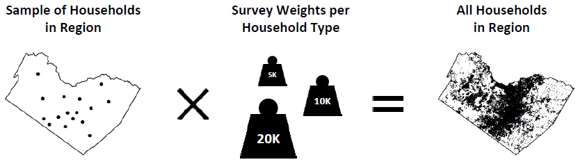
Figure 20. Expanding Household Samples to Represent All Households in a Region
For example, the regional household travel survey for Austin, Texas could be used to estimate the total amount of time traveled by walking for the five-county region. The survey sample is comprised of 3,000 households and 8,100 persons and can be expanded to represent the population of the study area by applying the survey weights. To do so, the total duration of trips by mode must be enumerated per household type, as defined in the survey stratification. The totals then must be multiplied by their corresponding survey weight to equal the total daily duration of trips by mode for the entire study area. The result is an estimated total of 189,256 daily walk trips with an average trip duration of 16 minutes equaling approximately 50,437 hours of walking per weekday.
The main limitations of region household travel surveys include their high cost and expertise required to process and analyze the survey data. The data may not be publically available due to survey respondent privacy concerns.
The Areawide Non-Motorized Exposure Tool described here makes it easier for practitioners to obtain and summarize nationwide travel survey data to estimate pedestrian and bicyclist exposure to risk at statewide and MPO area scales. The first part of the tool titled Statewide Exposure Estimates fills that gap between years when the NHTS is conducted by using the more current ACS data to estimate non-motorized exposure at the state-level. The second part of the tool titled MPO Area Exposure Estimates also uses NHTS and ACS data to estimate non-motorize exposure but for individual MPOs throughout the nationBoth parts of the tool produce annual non-motorized exposure estimates by mode for years 2009 to 2016 in terms of trips, miles of travel, and hours of travel for their respective areawide geography. The results are offered in tabular form along with graphics like the examples shown in Figure 21The following sections describe the tool's capabilities, as well as instructions on how to use the tool.
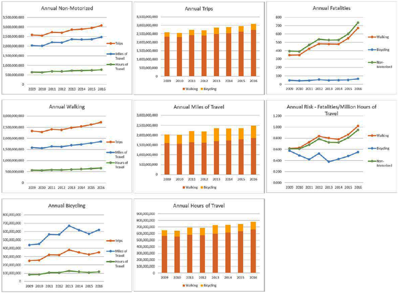
Figure 21. Annual Non-Motorized Exposure Estimates, Non-Motorized Fatalities, and Risk
The FHWA's Safety Performance Management (Safety PM) Final Rule currently requires each State DOT to report the number of non-motorized fatalities and serious injuries (without considering exposure). To understand the relationship between these crashes and non-motorized risk, exposure is desirable to help measure the magnitude of bicyclist and pedestrian vulnerabilityHowever, users should note that, at this time, the Safety PM Final Rule does not require non-motorized exposure to be reported or considered.
The Statewide Exposure Estimates component offers a method for practitioners to estimate statewide non-motorized exposure in order to calculate non-motorized risk. The tool provides the following exposure measure estimates for both bike and walk travel modes per state for the individual years 2009-2016:
The estimates are based on a combination of the 2009 NHTS and the U.SCensus Bureau's ACS data for each respective year. The 2009 NHTS total annualized trips per state are adjusted to better represent the selected year for analysis by using the more current ACS population and daily commute trip estimates (tables B01003 and B08301, respectively). The adjustment factors account for change in both population and the number of commute trips per mode over time. The population adjustment factor (AFpop,i) is based on the 2009 ACS population estimate since the NHTS data represent 2009It can be written as:
Where:
AFpop,i = Population adjustment factor in ith year (i = 2009 to 2016) for state
POPi = ACS population estimate in ith year for state
POP2009 = ACS population estimate in 2009 for state
In order to expand daily person commute biking and walking trips, the relationship between commute and total trips is required. The commute trip adjustment factor is based on the 2009 NHTS annualized person trips per person by mode (bike and walk) and the annualized ACS daily persons commuting by mode (bike or walk) for the selected year (i.e., ith year) for analysis. The equation is as follows:
Where:
AFCT = Commute trip adjustment factor by mode for state
PT2009 = NHTS annualized person trips by mode in 2009 for state
PC2009 = ACS daily persons commuting by mode in 2009 for state
The adjustment factors (AF) are applied to the selected year ACS commute trips per person by mode to provide estimated annual person trips:
Where:
PTi = Estimated annual person trips by mode (biking or walking) in ith year for state
PCi = ACS daily persons commuting by mode in ith year for state
AFpop,i = Population adjustment factor in ith year for state
AFCT,i = Commute trip adjustment factor by mode for state
Finally, to calculate the estimated total annual miles and hours traveled, the 2009 NHTS average trip durations and trip lengths per state were then applied to the total trips to estimate the amount of hours and miles traveled annually per mode for each state.
Where:
HTi = Estimated annual hours traveled by mode (biking or walking) in ith year for state
PTi = Estimated annual person trips by mode in ith year for state
TD2009 = 2009 NHTS average trip duration (in hours) by mode for state
MTi = Estimated annual miles traveled by mode in ith year for state
TL2009 = 2009 NHTS average trip length (in miles) by mode for state
Data sources for the above variables are as follows:
| Variable | Data Source |
|---|---|
| POPi & POP2009 | ACS 1-year estimate, table B01003 - Total Population |
| PCi & PC2009 | ACS 1-year estimate, table B08301 - Means Of Transportation To Work |
| PT2009 | 2009 NHTS |
| TD2009 | 2009 NHTS |
| TL2009 | 2009 NHTS |
This method assumes that the average trip durations and lengths remain constant between year 2009 and 2016 due to the lack of more current data. However, the tool does provide the user the option to input their own values if available In addition, the tool should be updated with the newly published 2017 NHTS data to produce the 2017 estimates based on current travel behavior data.
The NHTSA Fatality Analysis Reporting System (FARS) person data were used to calculate the total annual non-motorized fatalities per state from 2009 to 2016. The totals are provided in the spreadsheet tool along with total annual risk per state that is based on the total annual non-motorized fatalities per million hours of travel. The total annual non-motorized fatalities are defined as individuals classified as a bicyclist or pedestrian that sustained a fatal injury in a motor-vehicle crash. Â As of May 2018, the 2016 FARS data were incomplete. The data can be found online: https://www.nhtsa.gov/research-data/fatality-analysis-reporting-system-fars
The interface of the Statewide Exposure Estimates component is shown in Figure 22.
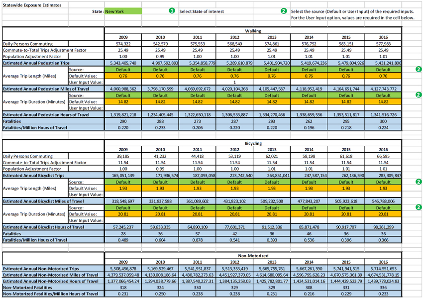
Figure 22. Interface of the Statewide Exposure Estimates Tool Component
The MPO Area Exposure Estimates component offers a method for practitioners to estimate MPO-wide non-motorized exposure for calculating non-motorized risk. The tool provides the following exposure measure estimates for both bike and walk travel modes per MPO for the individual years 2009-2016:
Non-motorized exposure estimates at the MPO level are derived from a combination of ACS and the 2009 NHTS. The Census data offers estimates at relatively small geographies that can be interpolated to the MPO leve. lThe 2009 NHTS data provides information on travel behavior for a sample of the travel public from around the nation and can be used to calculate average person trip rate, average trip length, and average trip duration per mode.
Total person trips by bike and walk can be estimated with a generalized 2009 person trip rate per mode applied to the total population of the year of interest and then annualized (365 days). The product is then adjusted to account for any change in the mode-specific commuting population between 2009 and the year of interest. However, this adjustment does not capture any change in non-motorized recreational travel that may be induced from communities investing in bicycle and pedestrian infrastructure. Total person trips are then be applied to the average trip length and average trip duration to equal total miles and total hours traveled per mode, respectively. It also important to note that any error in the 2009 NHTS estimates of walking or bicycling is carried through to the subsequent years.
The MPO-level estimated annual person trips by mode equation is as follows:
Where,
PTi = Estimated annual person trips by mode (biking or walking) in ith year for MPO
PTR2009Â = 2009 NHTS average daily person trip rate by mode for CBSA peer group
POPi = ACS 5-year population estimate in ith year for MPO
PCi = ACS 5-year daily persons commuting by mode estimate in ith year for MPO
PC2009Â = ACS daily persons commuting by mode 2009 for MPO
To calculate the estimated total annual miles and hours traveled, the 2009 NHTS average trip durations and trip lengths per MPO are applied to the total trips to estimate the amount of hours and miles traveled annually per mode for each MPO.
Where,
HTi = Estimated annual hours traveled by mode (biking or walking) in ith year for MPO
PTi = Estimated annual person trips by mode in ith year for MPO
TD2009Â = 2009 NHTS average daily person trip duration (in hours) by mode for CBSA peer group
MTi = Estimated annual miles traveled by mode in ith year for MPO
TL2009Â = 2009 NHTS average daily person trip length (in miles) by mode for CBSA peer group
Data sources for the above variables are as follows:
| Variable | Data Source |
|---|---|
| PTR2009 | 2009 NHTS |
| POPi | ACS 5-year estimate, table B01003 - Total Population |
| PCi & PC2009 | ACS 5-year estimate, table B08301 - Means Of Transportation To Work |
| TD2009 | 2009 NHTS |
| TL2009 | 2009 NHTS |
Several caveats do apply to this methodThe end user should keep in mind that the MPO-level estimates for their area are based on an estimated average for their CBSA (Core Based Statistical Area) peer group. Also, like the statewide tool, the MPO-level method assumes that the average trip durations and lengths remain constant between year 2009 and 2016 due to the lack of more current data. However, the tool does provide the user the option to input their own values if available.
The NHTSA FARS person data were used to calculate the total annual non-motorized fatalities per MPO from 2009 to 2016. The crashes were plotted in a GIS based on the coordinated provided and spatially joined the underlying MPO layerThe totals along with total annual risk per MPO that is based on the total annual non-motorized fatalities per million hours of travel are provided in the spreadsheet tool. The total annual non-motorized fatalities are defined as individuals classified as a bicyclist or pedestrian that sustained a fatal injury in a motor-vehicle crash. As of May 2018, the 2016 FARS data were incompleteThe data can be found online: https://www.nhtsa.gov/research-data/fatality-analysis-reporting-system-fars.
The interface of the MPO Area Exposure Estimates component is shown in Figure 23.
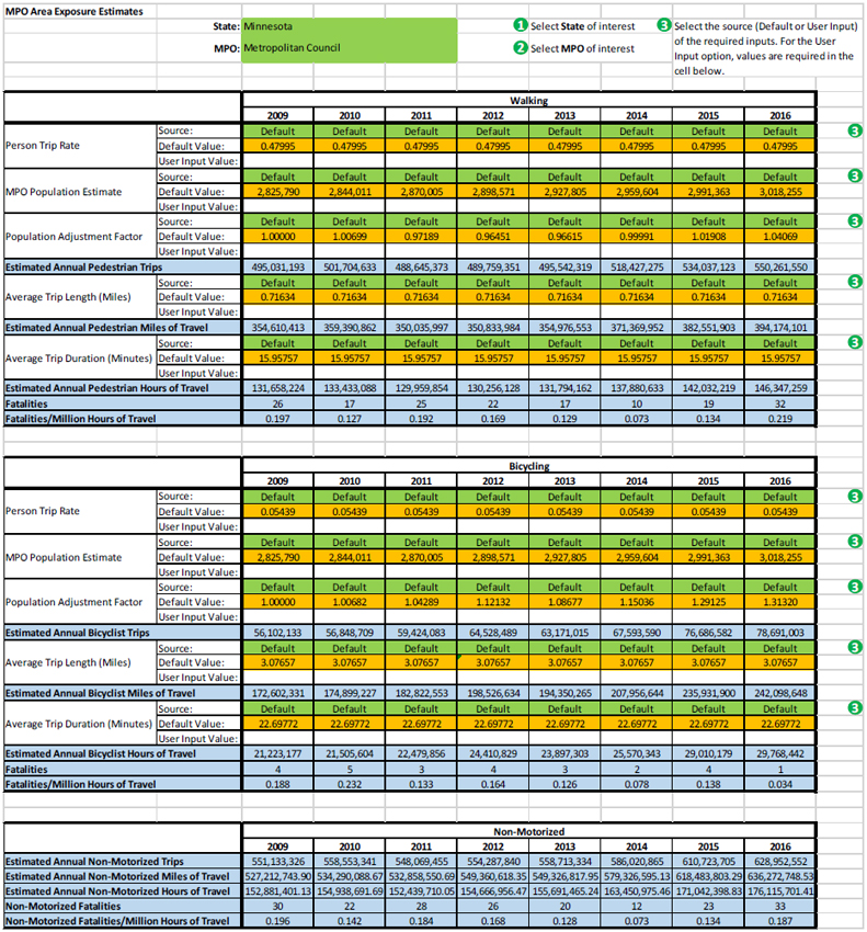
Figure 23. Interface of the MPO Area Exposure Estimates Tool Component
The Census does not offer data specific to MPO geographies; therefore, tract-level ACS Census data are used to provide the finest resolution to areal interpolate the population and commuter population for the MPOs. Only ACS 5-year estimates are available at the tract level; therefore, the estimates represent a given year within the five-year period as opposed to any individual year. 1- and 3-year estimates are unavailable due to inadequate ACS sample sizes at small geographies (i.e., tracts and counties). Figure 24 offers a visual comparison example of the Census Core-base Statistical Areas (CBSA), MPO and tract geographies for Memphis, TN.
Variables that require ACS data:
POPi = MPO population in ith year (derived through areal interpolation of tract-level ACS data)
PCi = MPO commuter population in ith year (derived through areal interpolation of tract-level ACS data)
PC2009Â = MPO commuter population in 2009 (derived through areal interpolation of tract-level ACS data)
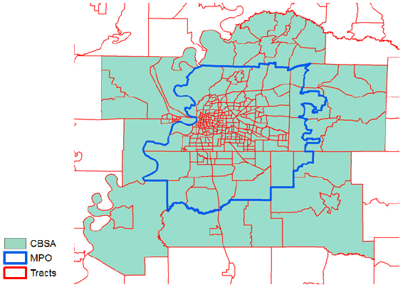
Figure 24. Geography Comparison
CBSA Peer Grouping Methodology: The 2009 NHTS survey data represent only a sample of the traveling public from both rural and urban areas. A portion of the 2009 NHTS data are labeled as being located within Census Core-base Statistical Areas (CBSA) that represent metropolitan areas. The CBSA geography is the smallest geography in the 2009 NHTS data and the only way to locate a portion of the survey sample.
The survey sample data are grouped by their CBSA as indicated in the original 2009 NHTS data to represent metropolitan areas around the nation. The CBSA metropolitan areas serve as proxies for MPOs in terms of developing of travel estimates from the 2009 NHTS; however, sample sizes vary between CBSAs and are possibly not statistically representative of the local populations. CBSAs are then grouped together based on 2009 ACS 1-year estimates for bicycle and walk commute percentages to increase samples sizes. Tables 22 (bike) and 23 (walk) list the ACS commute percentage ranges for the initial CBSA peer groupings along with their corresponding 2009 NHTS trip sample and the generalized travel estimates.
Generalized Travel Estimates Applied to MPOs: The 2009 NHTS survey data are used to generate an average person trip rate, average trip length (miles), and average trip duration (minutes) for bicycling and walking per CBSA grouping. These generalized travel estimates are applied to the MPOs that possess similar bicycle and walk commute percentages as their peer 2009 NHTS CBSAsThe MPOs area assigned a CBSAs peer grouping for every year between 2009 and 2016 based on the annual release of ACS 5-year estimates for bicycling and walking commute percentages. Refer to the Appendix for a list of the MPOs with their corresponding ACS population and commuter information along with their CBSA bike and walk grouping assignments.
In developing the generalized travel estimates, the NHTS survey weights are not applied because:
| CBSA Name | 2009 ACS Bike Commute Percentage | Quintile Grouping | 2009 NHTS Bike Trips | Average Person Trip Rate | Average Person Trip Length (miles | Average Person Trip Duration (minutes) |
|---|---|---|---|---|---|---|
| Memphis, TN-MS-AR | 0.02% | 1 | 531 | 0.00598 | 2.43 | 18.29 |
| Nashville-Davidson--Murfreesboro--Franklin, TN | 0.09% | |||||
| Charlotte-Gastonia-Concord, NC-SC | 0.11% | |||||
| Birmingham-Hoover, AL | 0.12% | |||||
| Dallas-Fort Worth-Arlington, TX | 0.13% | |||||
| Cincinnati-Middletown, OH-KY-IN | 0.18% | |||||
| San Antonio, TX | 0.18% | |||||
| Oklahoma City, OK | 0.20% | |||||
| Atlanta-Sandy Springs-Marietta, GA | 0.20% | |||||
| Kansas City, MO-KS | 0.21% | |||||
| Cleveland-Elyria-Mentor, OH | 0.22% | |||||
| Pittsburgh, PA | 0.24% | 2 | 609 | 0.00779 | 2.47 | 21.15 |
| Hartford-West Hartford-East Hartford, CT | 0.24% | |||||
| Louisville-Jefferson County, KY-IN | 0.26% | |||||
| Houston-Sugar Land-Baytown, TX | 0.27% | |||||
| Riverside-San Bernardino-Ontario, CA | 0.27% | |||||
| Providence-New Bedford-Fall River, RI-MA | 0.28% | |||||
| StLouis, MO-IL | 0.30% | |||||
| Richmond, VA | 0.31% | |||||
| Indianapolis-Carmel, IN | 0.32% | |||||
| Detroit-Warren-Livonia, MI | 0.32% | |||||
| Baltimore-Towson, MD | 0.33% | 3 | 662 | 0.00719 | 2.77 | 21.45 |
| Las Vegas-Paradise, NV | 0.34% | |||||
| Buffalo-Niagara Falls, NY | 0.35% | |||||
| Raleigh-Cary, NC | 0.36% | |||||
| New York-Northern New Jersey-Long Island, NY-NJ-PA | 0.40% | |||||
| Virginia Beach-Norfolk-Newport News, VA-NC | 0.41% | |||||
| Columbus, OH | 0.42% | |||||
| Milwaukee-Waukesha-West Allis, WI | 0.43% | |||||
| Orlando-Kissimmee, FL | 0.45% | |||||
| Rochester, NY | 0.50% | |||||
| Chicago-Naperville-Joliet, IL-IN-WI | 0.57% | 4 | 1,406 | 0.00970 | 2.82 | 22.07 |
| Washington-Arlington-Alexandria, DC-VA-MD-WV | 0.57% | |||||
| Miami-Fort Lauderdale-Pompano Beach, FL | 0.61% | |||||
| San Diego-Carlsbad-San Marcos, CA | 0.62% | |||||
| Jacksonville, FL | 0.64% | |||||
| Tampa-St Petersburg-Clearwater, FL | 0.70% | |||||
| Denver-Aurora-Broomfield, CO | 0.72% | |||||
| Austin-Round Rock, TX | 0.72% | |||||
| Philadelphia-Camden-Wilmington, PA-NJ-DE-MD | 0.73% | |||||
| Minneapolis-St Paul-Bloomington, MN-WI | 0.86% | |||||
| Los Angeles-Long Beach-Santa Ana, CA | 0.86% | 5 | 1,430 | 0.01227 | 3.08 | 22.70 |
| Salt Lake City, UT | 0.87% | |||||
| Phoenix-Mesa-Scottsdale, AZ | 0.91% | |||||
| Seattle-Tacoma-Bellevue, WA | 0.92% | |||||
| New Orleans-Metairie-Kenner, LA | 0.96% | |||||
| Boston-Cambridge-Quincy, MA-NH | 1.03% | |||||
| San Jose-Sunnyvale-Santa Clara, CA | 1.43% | |||||
| San Francisco-Oakland-Fremont, CA | 1.54% | |||||
| Sacramento--Arden-Arcade--Roseville, CA | 1.62% | |||||
| Portland-Vancouver-Beaverton, OR-WA | 2.13% |
| CBSA Name | 2009 ACS Walk Commute Percentage | Quintile Grouping | 2009 NHTS Walk Trips | Average Person Trip Rate | Average Person Trip Length (miles) | Average Person Trip Duration (minutes) |
|---|---|---|---|---|---|---|
| Orlando-Kissimmee, FL | 0.97% | 1 | 10,692 | 0.07503 | 0.70 | 14.35 |
| Nashville-Davidson--Murfreesboro--Franklin, TN | 1.10% | |||||
| Birmingham-Hoover, AL | 1.30% | |||||
| Memphis, TN-MS-AR | 1.33% | |||||
| Richmond, VA | 1.34% | |||||
| Dallas-Fort Worth-Arlington, TX | 1.40% | |||||
| Atlanta-Sandy Springs-Marietta, GA | 1.41% | |||||
| Tampa-StPetersburg-Clearwater, FL | 1.43% | |||||
| Kansas City, MO-KS | 1.48% | |||||
| Raleigh-Cary, NC | 1.51% | |||||
| Houston-Sugar Land-Baytown, TX | 1.55% | |||||
| Indianapolis-Carmel, IN | 1.57% | 2 | 6,023 | 0.09039 | 0.67 | 14.55 |
| Jacksonville, FL | 1.58% | |||||
| Charlotte-Gastonia-Concord, NC-SC | 1.58% | |||||
| StLouis, MO-IL | 1.64% | |||||
| Detroit-Warren-Livonia, MI | 1.65% | |||||
| Louisville-Jefferson County, KY-IN | 1.66% | |||||
| Oklahoma City, OK | 1.66% | |||||
| Austin-Round Rock, TX | 1.77% | |||||
| Miami-Fort Lauderdale-Pompano Beach, FL | 1.77% | |||||
| Las Vegas-Paradise, NV | 1.78% | |||||
| Phoenix-Mesa-Scottsdale, AZ | 1.80% | 3 | 7,854 | 0.08853 | 0.73 | 15.93 |
| Sacramento--Arden-Arcade--Roseville, CA | 1.84% | |||||
| San Antonio, TX | 2.02% | |||||
| Riverside-San Bernardino-Ontario, CA | 2.03% | |||||
| San Jose-Sunnyvale-Santa Clara, CA | 2.13% | |||||
| Columbus, OH | 2.14% | |||||
| Denver-Aurora-Broomfield, CO | 2.15% | |||||
| Cincinnati-Middletown, OH-KY-IN | 2.16% | |||||
| Hartford-West Hartford-East Hartford, CT | 2.19% | |||||
| Cleveland-Elyria-Mentor, OH | 2.25% | |||||
| Minneapolis-St Paul-Bloomington, MN-WI | 2.26% | 4 | 13,552 | 0.10889 | 0.72 | 15.96 |
| Salt Lake City, UT | 2.27% | |||||
| Virginia Beach-Norfolk-Newport News, VA-NC | 2.40% | |||||
| New Orleans-Metairie-Kenner, LA | 2.59% | |||||
| Los Angeles-Long Beach-Santa Ana, CA | 2.63% | |||||
| Providence-New Bedford-Fall River, RI-MA | 2.79% | |||||
| San Diego-Carlsbad-San Marcos, CA | 2.80% | |||||
| Baltimore-Towson, MD | 2.85% | |||||
| Milwaukee-Waukesha-West Allis, WI | 2.88% | |||||
| Buffalo-Niagara Falls, NY | 3.10% | |||||
| Chicago-Naperville-Joliet, IL-IN-WI | 3.17% | 5 | 14,211 | 0.14297 | 0.68 | 14.50 |
| Portland-Vancouver-Beaverton, OR-WA | 3.17% | |||||
| Washington-Arlington-Alexandria, DC-VA-MD-WV | 3.21% | |||||
| Rochester, NY | 3.37% | |||||
| Seattle-Tacoma-Bellevue, WA | 3.57% | |||||
| Pittsburgh, PA | 3.71% | |||||
| Philadelphia-Camden-Wilmington, PA-NJ-DE-MD | 3.75% | |||||
| San Francisco-Oakland-Fremont, CA | 4.40% | |||||
| Boston-Cambridge-Quincy, MA-NH | 5.12% | |||||
| New York-Northern New Jersey-Long Island, NY-NJ-PA | 6.28% |
The following section offers details on how to the manually extract data from the ACS and NHTS sources. These data sources offer a variety of additional demographic and travel behavior information that may be of value to safety analysis projects or outreach efforts.
ACS provides pedestrian and bicycle commuting estimates in geodatabase and CSV formats.7 Data are available for different measures related to pedestrian and bicycle commutingUsers can download data based on their requirementsTo get estimate the number of workers that commute to work by walking or bicycling, four major variables can be used (see Table 24).
| Census Code | Variable Name |
|---|---|
| B08301e18 | Means of Transportation to Work: Bicycle: Workers 16 years and over -- (Estimate) |
| B08301m18 | Means of Transportation to Work: Bicycle: Workers 16 years and over -- (Margin of Error) |
| B08301e19 | Means of Transportation to Work: Walk: Workers 16 years and over -- (Estimate) |
| B08301m19 | Means of Transportation to Work: Walk: Workers 16 years and over -- (Margin of Error) |
To create maps, users can use ESRI ArcGIS software to join TIGER/Line (Topologically Integrated Geographic Encoding and Referencing) shapefile with the ACS data tables.
With the following steps, users can determine bicycle-commuting estimates for census tracts in TexasIt is important to note that manual data extraction requires expertise in ArcGIS tool.
1: Download 2011-2015 ACS Data from U.SCensus8 (see Figure 25).
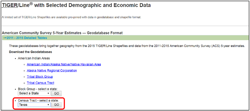
Figure 25. ACS Data for Texas
2: By using ArcMap 10.3, users can join ACS shapefile with ACS commuting data provided in the geodatabaseShapefile's variable 'GEOID' is required to be joined with 'GEOID' variable in ACS commuting data (see Figure 26).
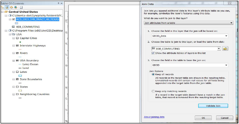
Figure 26. Joining of ACS Commuting Data with ACS Shapefile Data
3: Export data to text file format from the joined ACS shapefile attribute table.
4: To generate a choropleth map (see Figure 27), users need to follow the following steps:
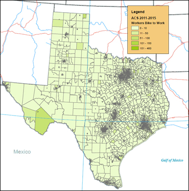
Figure 27. Map for Bicycle Commuting in Texas Census Tracts
The following section highlights NHTS online tools that provide relevant pedestrian and bicyclist travel summaries at the state and CBSA geographies based on the NHTS data files as presented in Table 25.
Since these data are collected via a survey, and not a census, they must be weighted according to ACS demographic information to represent the entire population and produce valid estimates. Survey weights for households and persons are available for all useable households in the NHTS databases.
The 2009 and 2017 NHTS national sample datasets (i.e., adjusted for oversampling due to add-ons) offer the ability to estimate non-motorized travel exposure by person trips at the state level. Figure 28 shows the online analysis tool with the total annual person trips by mode per state from the 2009 NHTS. The tool provides choropleth maps of 2009 NHTS person trips per state with drill-down capability to state statistics on trips, mode, and purpose. For example, Colorado produced approximately 7 billion person trips in 2009 with 9.7% (approximately 675 million) being walking trips.
| Data Files | Information Included | Record Level | ID Variables | Weight Variables |
|---|---|---|---|---|
| Household | Data unique to a householdExample questions from interview sections:
|
One record per household unit | HOUSEID | WTHHFIN |
| Person | Data determined once for each completed person interview Example questions from interview sections:
|
One record per person | HOUSEID PERSONID |
WTPERFIN |
| Vehicle | Data relating to each of the household's vehiclesExample questions from interview section:
|
One record per vehicle, if present | HOUSEID VEHID |
WTHHFIN |
| Travel Day Trip | Data about each trip the person made on the household's randomly-assigned travel dayExample questions from interview section
|
One record per travel day person trip | HOUSEID PERSONID TDTRPNUM |
WTTRDFIN |
Sources: 2009 NHTS Users Guide V2, page 6-2 and 2017 NHTS Users Guide, page 53

Figure 28. State-Level Annual Person Trips in NHTS Online Analysis Tool
Another online analysis tool based on the 2009 and 2017 NHTS national sample datasets is the table designer shown in Figure 29 and Figure 30. The table designer tools allow users to build customized data tabulations quickly and easilyThe tabulation outputs are offered in either HTML, Excel, or CSV formats.
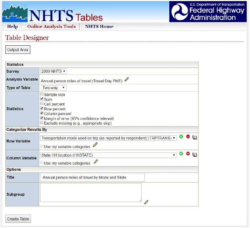
Figure 29. Table Designer Custom Query Tool for the 2009 NHTS
The NHTS attributes can also be tabulated for various census-based geographies, such as state, CBSA, and rural/urban (http://nhts.ornl.gov/2009/pub/UsersGuideClaritas.pdf)For example, the exposure measure of annual person miles of travel can be calculated by mode per state with these toolsTable 26 shows that in 2017 Arizona generated approximately 114 billion person miles of travel, of which 0.5% (approximately 585 million) were by walking.
Table 26. 2017 NHTS Annual Person Miles of Travel (millions) by Mode and State
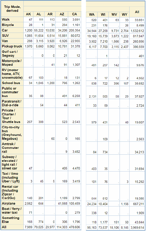
Source: Federal Highway Administration, 2017 NHTS
1 Rails-to-Trails Conservancy is developing nationwide seasonal adjustment factors in its Trail Modeling and Assessment Platform (T-MAP), as is Portland State in its PORTAL non-motorized count database↑
2 McKenzie, BModes Less Traveled—Bicycling and Walking to Work in the United States: 2008–2012 American Community Survey Reports2014↑
3 U.SCensus Bureau, A Compass for Understanding and Using American Community Survey Data: What General Data Users Need to Know, October 2008↑
4 U.SCensus Bureau, A Compass for Understanding and Using American Community Survey Data: What General Data Users Need to Know, October 2008↑
5 NCHRP Report 588: A Guidebook for Using American Community Survey Data for Transportation PlanningTransportation Research Board, Washington DC, 2007↑
6 Schneider, R.J., JVargo, and ASanatizadeh. Comparison of US Metropolitan Region Pedestrian and Bicyclist Fatality Rates, Accident Analysis and Prevention, Forthcoming, 2017↑
7 American FactFinder https://factfinder.census.gov/faces/nav/jsf/pages/index.xhtml↑
8 TIGER/Line® with Selected Demographic and Economic Data https://www.census.gov/geo/maps-data/data/tiger-data.html Accessed on Sept 29, 2017↑
| < Previous | Table of Contents | Next > |