U.S. Department of Transportation
Federal Highway Administration
1200 New Jersey Avenue, SE
Washington, DC 20590
202-366-4000
| < Previous | Table of Contents | Next > |
Step 8 in the scalable risk assessment process is to calculate risk values based on the outputs from previous steps. That is, Step 6 provides exposure estimates and Step 7 provides observed crashes, expected crashes, or additional risk indicators that are then used to calculate final risk values at the geographic scale chosen in previous steps.
Case studies are provided in this chapter to tie together the eight steps described in this guide. The case studies are based on actual examples of risk assessment for pedestrians and bicyclists.
The Michigan DOT partnered with the University of Michigan Transportation Research Institute to develop a risk assessment tool (http://www.cmisst.org/pedbike-risk-exposure/) for pedestrian crashes for all 83 counties throughout the state. Michigan DOT’s goal was to create a risk score, based on mapping crashes and the risk characteristics, for a defined area or network for the entire state of Michigan. We now present a fictional case example based on this project.
This case example focuses on pedestrian risk assessment to identify corridors in Detroit Michigan in need of countermeasures. Often the characteristics that make walking safe (or unsafe) persist over space. For example, along busy roads, land use features like business districts or the lack of lighting are often consistent over space. Due to this spatial continuity, transportation engineers often would like to improve the facilities in an entire corridor, not just one location.
| Steps | Explanation |
|---|---|
| Step 1: Define Use(s) of Risk Values | Network screening, Area Based |
| Step 2: Select Geographic Scale | Areawide->Network->Corridor |
| Step 3: Select Risk Definition | Definition 2: Expected Crashes |
| Step 4: Select Exposure Measure | Trips made |
| Step 5: Select Exposure Estimation Method | Demand Estimation ->Pedestrian Trip generation and flow models |
| Step 6: Estimate Exposure | Estimate binomial and logistic regressions |
| Step 7: Compile Other Required Data | |
| Step 8: Calculate Risk Values |
The MDOT engineers were interested in estimating pedestrian risks to identify corridors in need of countermeasures.
MDOT project team was interested analyzing risk at the corridor level.
The definition of risk combined various risk indicators to estimate the expected number of pedestrian-vehicle crashes.
The project team measured exposure in trips per day in a Pedestrian Analysis Zone (PAZ), which is a 400m x 400m unit of analysis. These units are aggregated up to the level of the corridor.
Demand Estimation –>Pedestrian Trip generation and flow models
The analytic method used a statewide travel survey, land-use data, and household characteristics to generate pedestrian trips at the PAZ level.
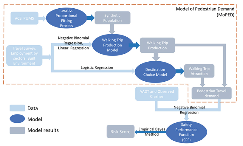
Figure 31. Step 5 Demand Estimation Using Pedestrian Trip Generation and Flow Models
The project team used the Michigan household travel survey (MTC III) to fit our trip production and destination choice models. We divided trips into five categories, namely home-based other (HBOther), home-based shopping (HBShopping), home-based school (HBSchool) and non-home-based other (NHBO) and non-home-based work (NHBW) and run the regression separately. We highlight the results for home based other (HBO) trips. For home-based trips, we estimate the number of trips per day at the household level using a negative binomial regression of the of the form,
Number of HB walking trips = f(number of households+household characteristics + built environment).
Below are representative regression results for the “home-based other” trip purpose.
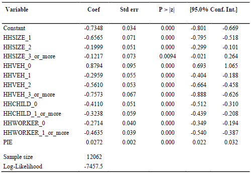
Figure 32. Pedestrian Trip Generation Model Results for home-based other trips
After completing all of the steps in the methodology, we obtained pedestrian exposure estimates. For more detailed information about the methodology, see (Cai et. al., 2018). Figure 33 shows the results for Wayne county Michigan where Detroit is located.
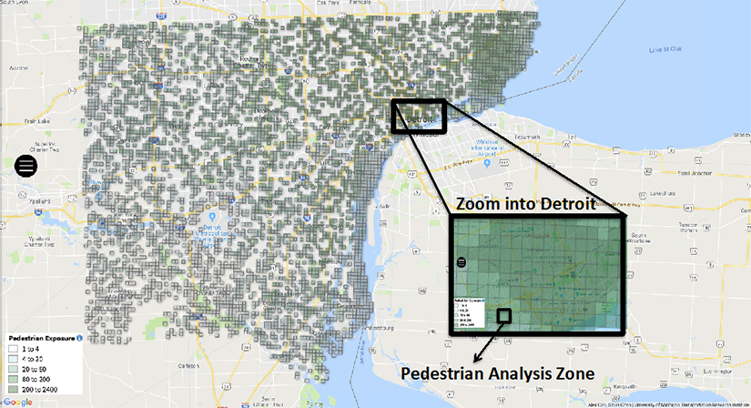
Figure 33. Daily pedestrian trips made per PAZ for Wayne county Michigan
The approach required many other data sources to calculate the risk values. The schematic below shows the various data sources used in the risk model.

Figure 34. Step 7: Compile other required data
We used the Empirical Bayes framework from the HSM to create customized safety performance functions (SPFs) for both bicyclist and pedestrians (Cai et al., 2018).
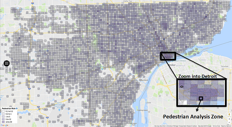
Figure 35. Risk measured as the expected number of crashes per PAZ
The MDOT engineers also wanted to analyze corridors. Thus we applied the Level-of-Service-of-Safety (LOSS) metric from the highway safety manual. LOSS divides the risk-scores of candidate areas into 4 categories based on its standard deviation from the average risk score (Kononov et al., 2003; Kononov et al., 2015). The areas in the highest quantile are the most dangerous for pedestrians. Figure 36 shows that LOSS map for pedestrian risk. In order to calculate the risk values of the corridors, we add together the risk score of each PAZ in the Gratiot corridor to arrive at a cumulative risk score of 50. The corresponding cumulative risk fir the Woodward corridor was 91.
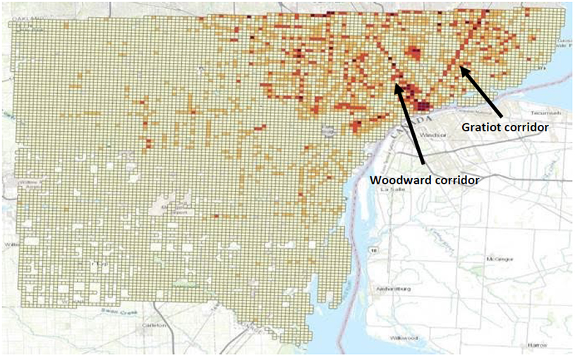
Figure 36. Level-of-Service-of-Safety (LOSS) map derived from the risk values
The scalable risk assessment methods were applied in Arizona as part of the Arizona DOT Bicycle Safety Action Plan as part of a statewide review of segments and intersection with a high priority for bicycle safety improvement projects.
| Steps | Explanation |
|---|---|
| Step 1: Define Use(s) of Risk Values | C. Network Screening - Facility-Based |
| Step 2: Select Geographic Scale | Facility Specific - Segments and Points (Intersections) |
| Step 3: Select Risk Definition | Definition 3: Additional Risk Indicators were used because bike count information is not feasible for the statewide network and the exposure estimation is not applicable to a statewide network |
| Step 4: Select Exposure Measure | Not applicable for Risk Indicators |
| Step 5: Select Exposure Estimation Method | Not applicable for Risk Indicators |
| Step 6: Estimate Exposure | Not applicable for Risk Indicators |
| Step 7: Compile Other Required Data | |
| Step 8: Calculate Risk Values |
The study team applied a network planning analysis approach to identify priority corridor locations and countermeasures to provide safety improvements for bicyclists. Emphasis was placed on providing safe conditions for bicycle travel all along a corridor (segment) and within the bicycle travel network. To apply this network analysis approach to the 2018 Bicycle Safety Action Plan Update for the Arizona State Highway System, high-crash intersections and segments and high-crash potential segments were grouped into Priority Locations. A Priority Location may consist of one or more high-crash segments, intersection, or high-crash potential segments. The high crash potential segments were identified through a risk assessment methodology. These Priority Locations comprise 94% of the high-crash segments, 100% of the high-crash intersections, and 74% of the high-crash potential segments.
The approach included an initial review of high bicycle crash locations on the Arizona State Highway System. These locations were identified using GIS and subsequently verified by visual inspection. The locations are separated into highway segments and intersections/interchanges. A high-crash intersection/interchange and segment location includes at least three bicycle crashes within the five-year period. In addition, bicycle count data were included where available for the intersection/interchange and segment location. The count data were from the recent Arizona DOT efforts to develop a bicyclist and pedestrian count strategy plan for the State Highway System. The purpose of the counts is to provide insight into the bicycle exposure on these selected high-crash locations.
A key element of improving bicycle safety in Arizona is to proactively identify locations where bicycle improvements are needed, leading to projects to address the need. This section introduces a risk assessment methodology that can assist ADOT in identifying state highway segments and intersections where investment can help to lower the risk of bicycle crashes. The proposed methodology is similar to the process used in the 2016 ADOT Pedestrian Safety Action Plan. The assessment methodology represents an approach through which high-probability segments can be identified and addressed before bicyclist/motor-vehicle crashes occur.
The methodology considers factors that are frequently identified as contributing factors or environmental/facility conditions that are common to bicycle crashes on the SHS. These factors are associated with the roadway facilities’ existing conditions that relate to the absence of sufficient bicycle accommodation and bicycle demand as data is available. Bicycle demand can be estimated based on the facilities’ proximity to specific land uses such as institutional areas that include schools, colleges, or universities, or being part of a known popular cycling route or corridor. Strava is a tool that can be used as a tool to help identify the popularity of cycling routes and corridors, although the Strava app data may be used more focused by recreational bicyclists.
Application of the methodology occurred through a GIS-based screening that utilized available statewide GIS data to identify and screen potential SHS locations where bicycle facilities should be considered, consistent with an established set of risk criteria. Note that interstates were excluded from the screening as the intent of this is application was to identify and direct resources to where they will be the most effective.
| Factor | Score |
|---|---|
| Operating Environment/Width of Roadway | |
| 6-Lane Highway | 6 |
| 4- or 5-Lane Undivided Highway | 3 |
| 2- or 3-Lane Undivided Highway | 2 |
| 2- or 3- or 4-Lane Divided Highway | 1 |
| Posted Travel Speed | |
| 50 mph or greater | 6 |
| 35-45 mph | 4 |
| 25-30 mph | 2 |
| 20 mph or less | 0 |
| Paved Effective Shoulder Width/Wide Curb Lane | |
| 0-4 feet | 6 |
| 4-8 feet | 0 |
| Bicyclist Exposure to Vehicles | |
| >7,500 ADT | 6 |
| 2,500-7,500 ADT | 3 |
| <2,500 ADT | 0 |
| Designated U.S. Bicycle Route (USBR) 90* | |
| Yes | 3 |
| No | 0 |
| Environment Type | |
| Urban | 6 |
| Rural | 3 |
*The USBR is not so much as risk factor, but is used to gain higher priority for improvements with the designation.
A scale was developed based on the distribution of the overall scores assigned to the SHS. The scale is defined in Table 29. A total of 31 higher-risk locations were identified and are shown in Figure 37.
| SCALE | RISK LEVEL |
|---|---|
| >20 | Higher Risk |
| 14-19 | Medium Risk |
| <13 | Lower Risk |
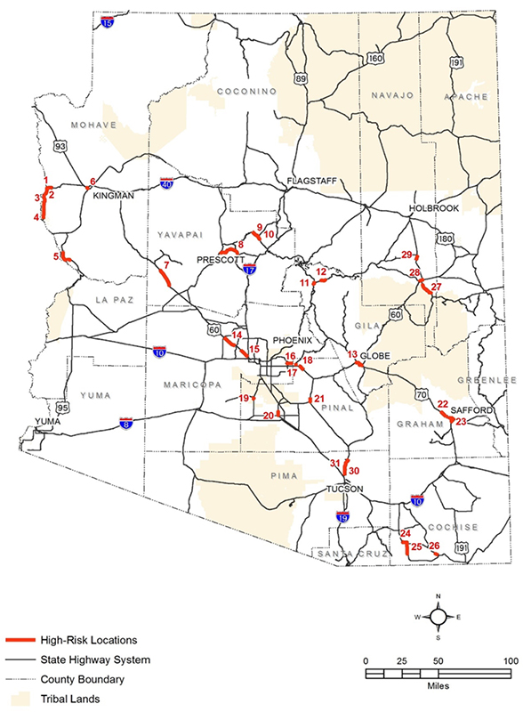
37. Higher-Risk Locations for Bicyclists on the Arizona State Highway System
| < Previous | Table of Contents | Next > |

