U.S. Department of Transportation
Federal Highway Administration
1200 New Jersey Avenue, SE
Washington, DC 20590
202-366-4000
Download Version
PDF [1.42 MB]
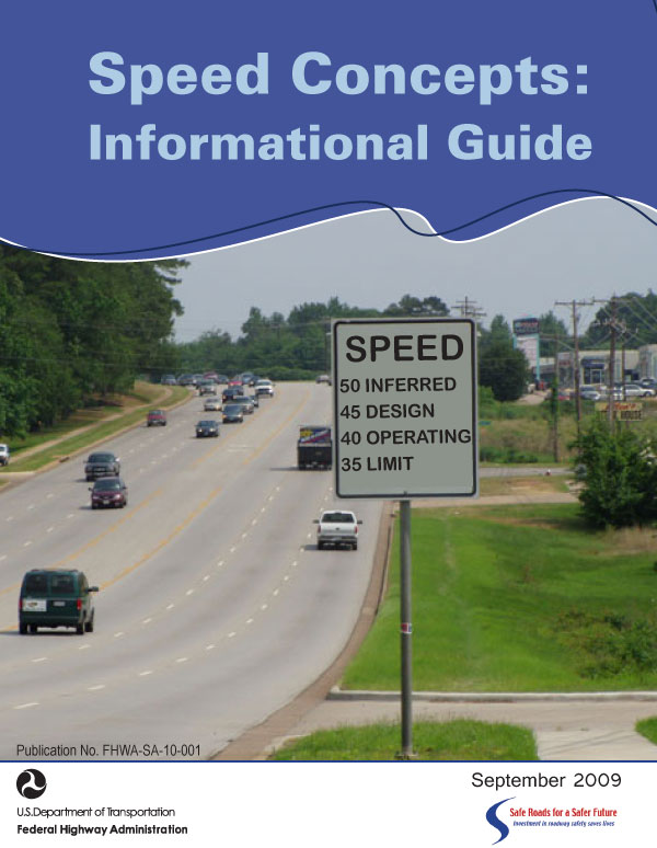
The speed at which drivers operate their vehicles directly affects two performance measures of the highway system—mobility and safety. Higher speeds provide for lower travel times, a measure of good mobility. However, the relationship of speed to safety is not as clear cut. It is difficult to separate speed from other characteristics including the type of highway facility. Still, it is generally agreed that the risk of injuries and fatalities increases with speed. Designers of highways use a designated design speed to establish design features; operators set speed limits deemed safe for the particular type of road; but drivers select their speed based on their individual perception of safety. Quite frequently, these speed measures are not compatible and their values relative to each other can vary. This guide discusses the various speed concepts to include designated design speed, operating speed, speed limit, and a new concept of inferred design speed. It explains how they are determined and how they relate to each other.
The purpose of this publication is to help engineers, planners, and elected officials to better understand design speed and its implications in achieving desired operating speeds and setting rational speed limits.
Joseph S. Toole
Associate Administrator,
Office of Safety,
Federal Highway Administration
This document is disseminated under the sponsorship of the U.S. Department of Transportation in the interest of information exchange. The U.S. Government assumes no liability for the use of the information contained in this document. This report does not constitute a standard, specification, or regulation.
The U.S. Government does not endorse products or manufacturers. Trademarks or manufacturers’ names appear in this report only because they are considered essential to the objective of the document.
The Federal Highway Administration (FHWA) provides high-quality information to serve Government, industry, and the public in a manner that promotes public understanding. Standards and policies are used to ensure and maximize the quality, objectivity, utility, and integrity of its information. FHWA periodically reviews quality issues and adjusts its programs and processes to ensure continuous quality improvement.
1. Report No. FHWA FHWA-SA-10-001 |
2. Government Accession No. |
3. Recipient's Catalog No. |
|||
4. Title and Subtitle Speed Concepts: Informational Guide |
5. Report Date December 2009 |
||||
6. Performing Organization Code
|
|||||
7. Authors Eric T. Donnell, Ph.D., P.E; Scott C. Hines, Kevin M. Mahoney, D. Eng., P.E., Richard J. Porter, Ph.D., Hugh McGee, Ph.D., P.E. |
8. Performing Organization Report No. |
||||
9. Performing Organization Name and Address Thomas D. Larson Pennsylvania Transportation Institute Vanasse Hangen Brustlin, Inc. |
10. Work Unit No.
|
||||
11. Contract or Grant No. DTFH61-03-D-00105 |
|||||
12. Sponsoring Agency Name and Address Office of Safety |
13. Type of Report and Period Covered Report |
||||
14. Sponsoring Agency Code
|
|||||
15. Supplementary Notes: FHWA COTR: Edward Sheldahl, Office of Safety. |
|||||
16. Abstract Traffic speed is an important yet complex topic in the transportation engineering community. Furthermore, speed is of considerable interest to enforcement agencies, safety advocates, property owners, users of the transportation system, and the public at-large because of its perceived effect on crash risk. Each of these stakeholders perceives speed measures differently; therefore, many issues related to speed are either misunderstood or remain unanswered. The objectives of this guide is to:
|
|||||
17. Key Words Traffic speed, design speed, inferred design speed, operating speed |
18. Distribution Statement
|
||||
19. Security Classif. (of this report) Unclassified |
20. Security Classif. (of this page) Unclassified |
21. No. of Pages: 59 |
22. Price |
||
Form DOT F 1700.7 (8-72) - Reproduction of completed pages authorized
SI (Modern Metric) Conversion Factors
Traffic speed is a subject of considerable interest and importance to transportation and traffic enforcement agencies, safety advocates, motorists, non-motorist street and highway users (e.g., pedestrians and bicyclists), residential and commercial property occupants and the public at-large. Speed is a controversial and complex subject. Even after significant research, many questions remain unanswered about speed relationships. The labels "good" and "bad" are difficult to apply to a particular speed condition since these terms are subjective and based on preferences, which often vary amongst different individuals and stakeholder groups.
Speed is often regarded as an indicator or measure of two different transportation performance characteristics, mobility and safety. Higher speeds generally translate to lower travel times, an indication of good mobility. The relationship between speed and safety is complicated and unclear. There are very few points of consensus on the effects of speed on crash probability. One of the many complicating factors is that high-speed highways (e.g., Interstates) have low crash rates. However, since Interstate highways also have distinguishing design features (e.g., limited access control and wide clear zones), it is difficult to separate the effects of speed from other characteristics. There is general agreement that the risk of injuries and fatalities increases with speed. So, even without a complete understanding, we know that conflicts can develop between the mobility and safety objectives.
Individual vehicle speeds are selected by drivers, a very large (over 200 million in the U.S.) and diverse population. They interpret and respond to signals, both explicit and implicit, in the driving environment. The roadway alignment, cross section, roadside, advisory speeds and speed limit are all elements of the driving environment that are thought to influence speed selection. Our knowledge is limited on how speed is affected by specific features, individually and in combination. However, it is known that different information sources (e.g., speed limit and roadway geometry) often send drivers different signals on appropriate speed. Speed management principles and techniques can be applied to clarify and unify the information being provided to drivers and to balance safety and mobility objectives.
The purpose of this publication is to help engineers, planners, and elected officials to better understand design speed and its implications in achieving desired operating speeds and setting rational speed limits. It answers the following questions:
This document is written such that it can be understood by a broad audience of interested readers. Extensive background knowledge is not needed. As a result, some subjects are not covered with the depth or precision customary in specialized research publications on speed-related subjects.
The following terms and abbreviations are commonly used in speed literature and discussions. Other references may use or define these terms somewhat differently than as defined below and used in this publication.
15th percentile speed – the speed at or below which 15 percent of vehicles travel. Also, see Speed distribution.
85th percentile speed – the speed at or below which 85 percent of vehicles travel. Also, see Speed distribution.
A – abbreviation for the algebraic difference in vertical alignment grades, in percent.
AASHTO – abbreviation for the American Association of State Highway and Transportation Officials.
Advisory speed – a speed below the speed limit that is recommended for a section of highway. The advisory speed is normally determined through an engineering study that considers highway design, operating characteristics and conditions. Advisory speeds are displayed on warning signs in speed values that are multiples of 5 mph. Advisory speeds cannot be enforced.
Designated design speed – the speed established as part of the geometric design process for a specific segment of roadway.
e – abbreviation for superelevation rate.
f – abbreviation for side friction factor.
FHWA - abbreviation for the Federal Highway Administration, an operating agency of the U. S. Department of Transportation.
g –force of gravity
Green Book – A Policy on Geometric Design of Highways and Streets (1) as published by AASHTO.
IHSDM – abbreviation for the Interactive Highway Safety Design Model, a collection of software tools that can be used to evaluate the safety and operational effects of geometric designs for two-lane rural highways.
Inferred design speed – the maximum speed for which all critical design-speed-related criteria are met at a particular location.
K – abbreviation for the rate of vertical curvature.
L – abbreviation for the length of vertical curve.
Mean speed - the summation of the instantaneous or spot-measured speeds at a specific location of vehicles divided by the number of vehicles observed. It is a common measure of central tendency.
MUTCD - abbreviation for the Manual on Uniform Traffic Control Devices.
NHTSA - abbreviation for the National Highway Traffic Safety Administration, an operating agency of the U. S. Department of Transportation.
Operating speed - the speeds at which vehicles are observed operating during free flow conditions. Free flow speeds are those observed from vehicles whose operations are unimpeded by traffic control devices (e.g., traffic signals) or by other vehicles in the traffic stream. The 85th percentile of the distribution of observed speeds is the most frequently used measure of the operating speed.
Posted speed – one of two speed limit types (statutory speed is other type); the maximum lawful vehicle speed for a particular location as displayed on a regulatory sign. Posted speeds are displayed on regulatory signs in speed values that are multiples of 5 mph.
R – abbreviation for horizontal curve radius.
Side friction – the lateral force developed between the tires and the roadway as a vehicle traverses a horizontal curve, expressed as a dimensionless coefficient of vertical force imposed by the vehicle’s weight.
SSD – abbreviation for the stopping sight distance.
Sight distance – the length along a roadway over which a driver has uninterrupted visibility – this is known as available sight distance. Different minimum sight distance design criteria exist for various operations and maneuvers, including stopping sight distance, passing sight distance and intersection sight distance.
Speed deviation – sometimes used to indicate Standard deviation of speed (see definition). Also, see Speed distribution.
Speed distribution – an arrangement of speed values showing their observed or theoretical frequency of occurrence.
Speed limit – the maximum lawful vehicle speed for a specific location. There are two types of speed limits, posted speed and statutory speed, definitions of each are provided.
Speed zone – a speed limit established on the basis of an engineering study for a particular section of road, for which the statutory speed limit is not appropriate.
Standard deviation of speed – a statistical measure (standard deviation) of the spread in values, applied to speeds. Also, see Speed distribution.
Statutory speed – one of two speed limit types (posted speed is other type). Numerical speed limits (e.g., 25 mph, 55 mph), established by state law that apply to various classes or categories of roads (e.g. rural expressways, residential streets, primary arterials, etc.) in the absence of posted speed limits.
USLIMITS version 2.0 - a web-based expert speed zoning software advisor.
Traffic speeds are relevant and of interest to nearly everyone. Our preferences and judgments of appropriate speed are strongly influenced by setting and perspective. The speed we prefer as a driver or passenger traveling long-distance along a rural Interstate highway is much different than what we prefer as a pedestrian crossing an urban street. Context is everything.
Speeds have fuel consumption, emissions and traffic noise consequences. Although these are important matters, most of the public interest and agency actions related to traffic speeds involve consideration of mobility and safety.
Speed is used directly and indirectly as a measure of mobility. For motorists, shippers and the commercial transportation industry, high operating speeds are considered desirable. Several other mobility measures (e.g., delay and travel time) are also linked to speed. For example, travel time along a specified route can be determined on the basis of distance and average speed. For this reason, facilities that emphasize mobility (e.g., Interstate highways and other freeways) accommodate high speed.
The effects of speed on safety are complex and only partially known. Despite a long and sustained research effort, only a limited number of consistent and reliable speed-safety relationships have been established, including:
A clear understanding of how speed affects safety has also been obscured by the use of different speed-related indicators and a wide range of study methods. Different studies have evaluated the safety effects of speed limits, operating speeds and design speed, with some studies making the unsubstantiated assumption that these characteristics are related to each other. Many of the speed related studies are based on data from high-speed highways. Too often, the results and conclusions of these studies are inappropriately applied to all roads and streets. Despite the complexity and challenge of understanding speed-safety relationships, useful research conclusions have been reached. Key research studies and conclusions are summarized below.
There is clear and convincing evidence that crash severity increases with individual vehicle speed. This finding is supported by theory and statistical analysis.
A vehicle’s kinetic energy is proportional to its velocity squared. When a crash occurs, all or part of the kinetic energy is dissipated, primarily through friction and mass deformation. As kinetic energy increases exponentially with speed, so does the potential for mass deformation, including humans that are inside and outside of the vehicle. Analysis of crash statistics (2) have shown that the probability of being injured in a crash increases as the change in speed at impact increases, particularly when this change in speed occurs over a short time duration.
A direct and positive relationship has been found between speed and the severity of pedestrian injury in vehicle-pedestrian crashes. The results of one United Kingdom study (3) are shown in the second column of table 1. A different study (4), conducted in the United States, also found a positive correlation between speed and severity of pedestrian injuries. The results, stratified by pedestrian age group are presented in columns three through five of table 1.
Table 1. Probability of pedestrian death resulting from various vehicle impact speeds.
Vehicle speed (mph) |
Probability of pedestrian fatality |
Probability of pedestrian fatality age = 14 (%)** |
Probability of pedestrian fatality age 15 to 59 (%)** |
Probability of pedestrian fatality age = 60 (%) ** |
20 |
5 |
1 |
1 |
3 |
30 |
45 |
5 |
7 |
62 |
40 |
85 |
16 |
22 |
92 |
*Source: Ref (3); ** Source: Ref (4)
A number of technical and engineering techniques are closely associated with traffic speeds. The designed driving environment consists primarily of infrastructure and traffic control devices. The geometric design process is used to define the location and dimensions of road and street infrastructure which consists of the horizontal and vertical alignment, cross section features, intersection type and all the associated details. Traffic control devices are used to regulate, warn and guide drivers through the use of signs, traffic signals, pavement markings and other devices.
Geometric design is an engineering discipline that attempts to account for interactions between drivers, infrastructure and vehicles. The techniques and criteria reflect both theoretical and practical considerations and evolve as new reliable research conclusions are reached. This section of the guide introduces and summarizes several technical topics and techniques that are closely related to speed.
The design speed is a selected speed used to determine the various geometric design features of the roadway (1). The historical evolution of the design speed definition has been well documented in NCHRP Report 504 (5). The design speed concept was first proposed in 1936 as "the maximum reasonably uniform speed which would be adopted by the faster driving group of vehicle operations, once clear of urban areas (6)." The American Association of State Highway Officials (AASHO) accepted a modified definition of design speed in 1938 as "the maximum approximately uniform speed which probably will be adopted by the faster group of drivers, but not, necessarily, by the small percentage of reckless ones (7)." Beginning with the 1954 version of A Policy on Geometric Design of Rural Highways, the definition of the design speed was "the maximum safe speed that can be maintained over a specified section of highway when conditions are so favorable that the design features of the highway govern. (8)." Inclusion of the "maximum safe speed" was included in the design speed definition until release of the 2001 version of the AASHTO Green Book. Removal of "the maximum safe speed" from the design speed definition was proposed in 1997 as a result of NCHRP Report 400 (9). It was recognized that operating speeds can be greater than the design speed, and the term safe was removed to avoid the perception that speeds greater than the design speed were "unsafe" (5). The revised definition as a result of NCHRP Report 400 is the definition that is presented at the beginning of this section, and is the definition used today. For the purposes of this informational guide, the design speed concept described in this section is referred to as the "designated design speed." The designated design speed is used explicitly for determining minimum values for highway design such as horizontal curve radius and sight distance. The designated design speed is typically included within design documentation and is often shown on the cover sheet of design plans.
A second design speed term is also used in this informational guide. It is referred to as the "inferred design speed." Inferred design speed is applicable only to features and elements that have a criterion based on (designated) design speed (e.g., vertical curvature, sight distance, superelevation). The inferred design speed of a feature will be different than the designated design speed when the actual value is different than the criterion-limiting (minimum or maximum) value. The inferred design speed for a radius-superelevation combination is the maximum speed for which the limiting speed-based side friction value is not exceeded for the designed rate of superelevation and the inferred design speed (determined through an iterative process). The inferred design speed for a horizontal curve may also be limited by horizontal offsets to sight obstructions on the inside of a horizontal curve. The inferred design speed for a crest vertical curve is the maximum speed for which the available stopping sight distance is not exceeded by the required stopping sight distance. The inferred design speed may also be limited by a combination of lane width and average daily traffic. The inferred design speed can be greater than, equal to, or less than the designated design speed.
To maintain vehicle paths and avoid conflicts, drivers need visibility of road and traffic conditions. Drivers continuously and (after a certain level of driving experience is gained) subconsciously process visual information through observation, interpretation and responsive action. Visibility needs are related to the operating environment and vehicle speeds. These are the key factors used in developing geometric criteria for sight distance. The Green Book identifies four types of sight distance: decision, intersection, passing (on two-lane roads) and stopping and provides guidance on where each type is recommended. The Green Book establishes minimum design values for sight distance and above minimum values are encouraged where feasible. As a result, the inferred design speed resulting from the highway geometric design process (i.e., actual roadway geometry that is constructed) is often higher than the designated design speed.
The methods of determining the criterion for a particular situation are also included in the Green Book and are related to speed. A set of assumptions, usually based on research or practical experience, are incorporated into the criteria. One of the key assumptions relates to the object or condition that should be seen. In the case of passing sight distance, the object is a vehicle approaching the passing vehicle in the same lane and opposite direction. The assumption is that the approaching vehicle is a passenger car and the object is assumed to be 3.5 feet above the pavement elevation. This is one of many assumptions used to formulate the relationship between speed and passing sight distance criteria.
Stopping sight distance should be provided along the entire length of every road and street. In that sense, it is the most common type of sight distance. The first and second columns in table 2 indicate the relationship between design speed and the Green Book stopping sight distance criteria on relatively level roadways. The criteria assume a driver perception-reaction time of 2.5 seconds, driver eye height of 3.5 feet and an object height (i.e., tail lights of another vehicle) of 2.0 feet. The assumptions for driver eye height and tail light height reflect the 5th percentile statistics (9). This means that 95 percent of vehicles have a driver eye height and tail light height greater than these values. The assumed perception-reaction time exceeds the 90th percentile driver reaction time. However, normal perception-reaction times vary from about 0.75 to 1.5 seconds (10) depending on the alertness, fatigue level, alcohol consumption, and age of the driver.
Table 2. Comparison of stopping sight distance requirements for various conditions.
Design speed (mph) |
AASHTO design stopping sight distance criteria (feet) |
Estimated stopping sight distance for mean driver |
Estimated stopping sight distance for dry roadway conditions |
15 |
80 |
40 |
75 |
20 |
115 |
60 |
110 |
25 |
155 |
80 |
150 |
30 |
200 |
105 |
190 |
35 |
250 |
135 |
235 |
40 |
305 |
165 |
285 |
45 |
360 |
200 |
340 |
50 |
425 |
235 |
400 |
55 |
495 |
275 |
465 |
60 |
570 |
320 |
535 |
65 |
645 |
365 |
605 |
70 |
730 |
415 |
680 |
75 |
820 |
465 |
765 |
80 |
910 |
520 |
850 |
Another assumption used in developing Green Book stopping sight distance criteria is that braking will result in a vehicle deceleration rate of 11.2 feet/second2 [0.35g]. This deceleration rate was developed through research in consideration of developments in vehicle technologies and driver performance. It also assumes that the friction provided by the driving surface is adequate to support this rate. Some vehicles with good tires on good pavement can brake at 0.85g or higher with most able to brake in emergency stops at 0.7g or better. Although most pavements provide adequate friction for the assumed deceleration rate, inclement weather conditions (e.g., snow and ice) may not. On wet pavement, most vehicles can stop at 0.4g or higher even with bald tires. The deceleration rate on ice [0.15g] and snow [0.22g] are lower (11). It has also been shown that heavy vehicles achieve the same deceleration rate as passenger cars on wet pavement when the heavy vehicle is equipped with antilock brakes (12). Since the AASHTO design criteria accounts for wet pavement and allows for controlled braking, it has been shown that the design stopping sight distance criteria are adequate for heavy vehicles.
In addition to the Green Book stopping sight distance design criteria shown in table 2, the third column is the estimated stopping sight distance based on the mean driver with a reaction time of 1.1 seconds and a vehicle deceleration rate of 17.71 ft/sec2 (9). This is intended to show how large the difference in required stopping sight distance is between the average driver and the design or 90th percentile driver. The final column in table 2 also shows the stopping sight distance required for the 90th percentile driver on dry roadway conditions. The design criteria assume that the available friction is that of a wet roadway. The difference between estimated wet and dry stopping sight distance is not based upon available friction, but drivers’ tendency to decelerate at a higher rate on dry pavement conditions. However, in an emergency stop, the difference between wet and dry stopping distance is due to friction.
Sight distance requirements also depend on the vertical alignment (or profile) of the roadway. On inclines (upgrades), the effect of gravity is to reduce vehicle speeds. Conversely, a vehicle descending a grade is being accelerated by gravity. For steep grades, uphill or down, gravity has a real and practical effect on the stopping sight distance. Generally, no adjustment to the base condition (level road) criteria is made for small grades (less than three percent), positive or negative.
Vertical curves are used to transition from one grade (i.e., slope in the direction of travel) to another. Figure 1 illustrates two types of vertical curves, crest and sag.
Figure 1. Crest and sag vertical curves.
The rate of change in grades affects both driver comfort and sight distance. Crest vertical curves can limit sight distance by restricting a driver’s line of sight, as shown in figure 2. In figure 2, the point of vertical curve (beginning point of curve), point of vertical intersection (intersection of initial and final grades), and point of vertical tangent (end point of curve) are shown as PVC, PVI, and PVT, respectively. The initial and final grades are G1 and G2, respectively. The unobstructed horizontal distance between the driver eye height (H1) and object height above the roadway surface (H2) defines the available stopping sight distance.
Sag vertical curves affect how headlight beams intersect the roadway and reveal an object as shown in figure 3. If a vertical curve is long enough to provide adequate sight distance, it will also provide adequate driver comfort.
Figure 2. Effect of crest vertical curves on sight distance.
Figure 3. Effect of sag vertical curves on sight distance.
Minimum rates of vertical curvature (K) are included in the Green Book for different categories of sight distance, design speed and vertical curve type (i.e., crest, sag). The minimum length of vertical curve can be determined by using these rates and equation 1, shown below.
Road and street alignments are comprised of two basic elements, curves and tangents. The most common type of horizontal alignment curve, and the only one discussed here, is the simple curve which has a single (constant) radius. Tangents are straight sections between curves.
The forces associated with vehicles and occupants moving along a curved path are more complicated than for a straight path. A vehicle and its contents (hereafter simplified to "vehicle") traversing a curved roadway at a constant speed are accelerating toward the center of the curve. This is known as centripetal acceleration. The magnitude of the acceleration is a function of the vehicle speed and radius of curvature.
A vehicle can only follow a circular roadway alignment if a centripetal force (Fc) is applied. The direction of this force is the same as the acceleration, toward the center of the curve. With some simplifying assumptions, equation 2 can be derived. The left side of the equation represents two external forces and the right side is the resulting acceleration.
The two left-hand side components represent superelevation and friction. Superelevation is another term for "banking" the roadway. As shown in figure 4, superelevation results in part of the vehicle’s mass being accelerated laterally, toward the low side of the banked section (the vehicle’s weight, W, is shown in Figure 4). Higher rates of superelevation increase the lateral acceleration provided by this component.
Figure 4. Cross section of vehicle on superelevated road.
It should be noted that superelevation and friction are "signed." They have magnitude and direction. Friction and superelevation do not necessarily act in the same direction. For purposes of this discussion, the positive direction is defined as toward the center of the curve. Negative superelevation is actually quite common. Think of a road with a normal crown (i.e., high point in center and sloping outward in both directions). If the normal crown is maintained through a curve, both sides have superelevation but with opposite signs. For a curve to the left, the right lane of a normal crown section has negative superelevation.
Friction usually, but not always, acts toward the center of the curve which has been defined as the positive direction. Exceptions occur, such as a vehicle traveling at low speed along a road with a high rate of superelevation. Once a road is constructed, the radius and superelevation (both direction and magnitude) are known and constant. The required side friction will vary with speed.
Drivers and other vehicle occupants moving on a turning roadway "feel" the side friction developed between the tire and pavement. It is often referred to as unbalanced lateral acceleration and is a direct indication of driver discomfort. A passenger (or driver) traveling along a curve at 70 mph will be less comfortable than one traversing the same curve at 55 mph. The use of friction factors in geometric design, particularly limiting or maximum values, is often misunderstood. Design criteria for horizontal curves (minimum radii, design rate of superelevation) are established so that maximum design side friction factors are not exceeded at the design speed. Maximum design side friction factors decrease with design speed. Values used in the 2004 Green Book are shown in figure 5. The values are established so that the friction required to maintain a vehicle’s path along the curved alignment will nearly always be achievable. Maximum design side friction factors are not determined solely as a matter of physics or engineering mechanics. Turning maneuvers become more demanding for drivers as the unbalanced lateral acceleration (side friction) increases. In recognition of this, human factors come into play in establishing maximum design side friction factors.
The term "comfort" is used to describe the human response to different levels of unbalanced lateral acceleration. The maximum design side friction factors were set so that unbalanced lateral acceleration levels do not cause discomfort to vehicle occupants. The values currently in use are based on research of passenger comfort (blindfolded passengers) conducted in the 1940s. Subsequent advancements in vehicle technologies call into question the validity of the historic research and its continued use for design and analysis purposes. This leads to two important conclusions. First, the maximum design side friction factors do not represent the limit of available friction based strictly on material properties and mechanics. Second, the research on human response to unbalanced lateral acceleration (i.e., demand friction) is dated and may no longer apply.
Observed speeds on horizontal curves routinely exceed designated design speeds. The maximum design side friction factors in use adequately accommodate the design speed under a wide range of conditions (i.e., related to tire, pavement and driver variability), including very poor conditions. Therefore, higher curve speeds can be attained under good conditions, and even average conditions. This condition is so prevalent that design values are suspected of being unrealistic or inappropriate.
Figure 5. Maximum side friction factors for various design speed.
Source: Ref (1)
Speeds are selected by the driver. Different drivers select different speeds, dependent upon many variables (vehicle limitations, roadway conditions, driver ability, etc.). No single speed value can accurately represent all the speeds at a particular location. A speed distribution (see definition in chapter 2) provides that information. Operating speeds have been found to be normally distributed (sometimes called a "bell-shaped curve"). This is fortunate since using that premise (probability is normally distributed) allows for some straightforward calculations. Even though a variable (e.g., speed, height) may be normally distributed, properties of the distribution may vary. Two different normal probability density functions are shown in figure 6. The vertical axis indicates the probability that the variable will take on the corresponding value on the horizontal axis. The speed distribution provides useful information but it is not a convenient way to describe speeds.
Figure 6. Normal probability distributions.
The unique properties of the normal probability distribution allow it to be conveniently described with just two characteristics, mean and standard deviation. These two characteristics also have practical importance for traffic speeds. Figure 7 includes plots of two different normal speed distributions. These distributions have the same mean but different standard deviations.
Figure 7. Examples of two normal probability distributions, operating speeds, same mean, different standard deviations.
For reasons stated elsewhere in this Informational Guide, the 85th percentile speed is a frequently used characteristic. The mean speed plus one standard deviation approximates the 85th percentile speed for a normally distributed sample of speeds. For an observed sample of speed data, determining the 85th percentile value is fairly easy, either manually (for relatively small samples) or a spreadsheet. To get a graphical sense of the 85th percentile speed, the cumulative distribution function can be plotted. An example is included as figure 8. To find the values associated with any Nth percentile (e.g., 25th, 60th or 85th percentile) level, find that percentile level on the vertical axis. Then move horizontally until the line representing the cumulative distribution function is intersected, project a line from that point down to the intersection with the horizontal axis. The value on the horizontal axis is associated with the Nth percentile. For the figure 8 example, the 85th percentile speed is 59 mph.
Speed profiles are a graphical representation of speed features plotted by location. Figure 9 is an example. Speed profiles are useful in studies and evaluations. The contents of speed profiles vary but features that are commonly included are the designated design speed, operating speed and posted speed limit; inferred design speed can be displayed as well.
Figure 8. Example cumulative distribution function, operating speeds.

Figure 9. Example speed profile.
Government agencies, mostly at the state, county and local levels, own and operate approximately four million miles of roads and streets in the U.S. Through road ownership and construction, statutes, traffic regulation and enforcement, government agencies create the physical and legal driving environment. Not all drivers respond in the same way to the same driving environment and these differences extend to speed selection. An understanding of speed issues requires some basic insights of agency functions and human behavior in a regulated environment.
Before a new road or street is built, plans are prepared by engineers. Except for minor streets and roads, the design process considers speed by adopting a designated design speed. The road is then constructed in accordance with the design plans and put into service for the motoring public, which is regulated by a set of laws and regulations, including an established speed limit. A more detailed description of these processes and their relationships is provided below.
Roadway geometry is one of the informal information sources that drivers interpret when selecting a speed. However, roadway geometry can provide deceptive, conflicting and confusing speed cues. This is unfortunate but true and because the existing network is so extensive, substantial modifications are often impractical.
The Green Book is the dominant reference publication for geometric design in the U.S. and its application involves selecting a "design speed." The definition of design speed has changed over time but the way it is used in the design process has not. The Green Book guidance on designating design speed does not address speed limits. The Green Book recommends that topography, anticipated operating speed, adjacent land use and functional classification be considered and as high a design speed as practical be selected, except for local streets. The selected (designated) design speed is used explicitly to determine:
Chapter 4 provides background for many of these speed-based design criteria. Some of these criteria, such as sight distance and vertical curvature, are related.
The Green Book provides minimum or limiting values for the design criteria. It also recommends "above-minimum design values should be used, where practical." The underlying rationale for this guidance is that above-minimum features will safely accommodate a condition beyond the assumed parameters. Historically, this was thought to be "conservative" and consistent with other engineering disciplines that use factors of safety to intentionally "over design" critical components. The direct effect of utilizing above-minimum design elements is that it affords drivers greater comfort to travel at higher speeds, and thereby leads to an "inferred" design speed greater than the designated design speed that may be inappropriate for surrounding conditions. A definition for "inferred design speed" is included earlier in this publication and will be referenced in the next paragraph. An example is provided on the following page to complement the definition and clarify the term’s meaning.
Frequently, roads and streets designed for a particular speed appear suitable for much higher speeds. Drivers read the road, not the design plans. Some roadway segments, such as a long straight section, look the same regardless of designated design speed. When these features are combined with over-designed speed sensitive features (i.e., from using above-minimum values as recommended by highway geometric design policy) the visible cues on appropriate speed may be in sharp contrast to the designated design speed. What was contemplated by the designer as a factor of safety (with respect to the designated design speed) is often negated by driver speed choice. The differing perceptions of speed by designer and driver are especially problematic where a single minimum-value feature (e.g., minimum radius curve) is located within a segment that generally has an inferred design speed much higher than the designated design speed. This condition is contrary to the design objective of "design consistency." However, the Green Book includes no specific design criteria for design consistency and the condition described technically complies with the geometric design policy.
Highway geometry is not the only cue drivers are receiving. Landscape, development, perceived conflicts, and intersections also contribute to the driver’s selection of speed. Just as selecting a design that is higher than necessary is inappropriate, it is also inappropriate to select a lower design speed if other cues will lead drivers to select a speed that is too high for the design geometry. We do not want the highway geometry to be a surprise to the driver.
Design policy recognizes that a wide range of performance levels exist amongst the large and diverse population of drivers. The need to integrate human performance and engineering design gives rise to another speed conundrum. Green Book criteria attempt to safely accommodate below-average driver proficiencies. Many drivers routinely drive at speeds faster than the speed limit and faster than other drivers. Overconfident drivers may come to believe they possess superior abilities and skills that enable them to operate safely at higher speeds.
Figure 10 illustrates an example relationship between speed, geometric design and differing levels of driver performance. Minimum stopping sight distance design criteria are based on several assumptions, as were previously discussed in chapter 4, including 2.5 seconds of driver perception-reaction time. The solid line in figure 10 is a plot of sight distance versus speed using a 2.5-second reaction time. The sight distance values coincide with Green Book stopping sight distance criteria, which are also listed in table 2. The broken-line plot is based on a reaction time of 1.5 seconds. Drivers do not use formulae to select their speeds; consequently some drivers drive faster because they feel capable of reacting quickly. However, the probability of dealing successfully with unexpected circumstances is reduced with higher speeds.
Figure 10. Sight distances corresponding to different reaction times.
The 85th percentile speed is used extensively in the field of traffic engineering and safety. Since the majority of drivers are considered reasonable and should be accommodated, some numerical definition for this segment of the driver population is needed. Over time, the 85th percentile driver (or speed) has been used to characterize reasonable and prudent behavior.
For a variety a reasons, including those summarized in this chapter, policy-compliant designs often appear adequate for speeds far above the designated design speed. The speed profile in figure 11 is an example of a case where the 85th percentile speed and posted speed exceed the designated design speed. These data were collected along an existing multi-lane highway in central Pennsylvania. The geometric features are in keeping with Green Book guidance recommending higher-than-minimum values for design features (e.g., vertical curve lengths, horizontal curve radii). The inferred design speed is substantially higher than the designated design speed. When the facility was first opened to traffic, the posted speed of 40 mph was "mismatched" with the geometric features. Based on a review of operating speeds, the speed limit was changed to 50 mph. Many researchers have noted that the design speed process has no systematic check for consistency between operating and design speeds. (13,14,15)
Figure 11. Speed profile with inferred design speed substantially exceeding designated design speed.
Even though the Green Book is the principal reference for geometric design, for two basic reasons there are many street and highway segments that do not conform to its current provisions:
Many city streets and some of the first freeways were designed prior to development of the design speed concept. Many designs were created without explicit consideration of vehicle speeds. AASHO, which was the predecessor to AASHTO, published its first design-related policies in the 1940s. The original AASHO policy used a design speed but it did not apply to urban streets. Over the years, AASHO, and then AASHTO, periodically updated and expanded its geometric design policy. As the policy became more complete (e.g., included procedures for urban streets) it reached its current status as the principal reference for designing U.S. roads and streets. When geometric design policy is updated, it is often not applied retroactively. In other words, facilities that were designed under an earlier policy are not automatically revised to meet the most current policy.
The use of AASHTO policy is only mandatory in the design of roads that are part of the National Highway System, which includes all Interstate highways and other selected arterial highways. For other roads and streets, state DOTs and local government units (i.e. counties, cities, boroughs, towns), have the discretion to develop and apply the geometric design process and criteria they consider most appropriate. State DOTs use design processes and criteria that are the same or similar to AASHTO’s. Local agency practice varies widely, with larger agencies typically adopting policies similar to their state DOTs, and therefore those of AASHTO. Local governments with limited roadway responsibilities (i.e., limited mileage and no arterials) may use very simple guidelines, such as those incorporated into subdivision regulations. These guidelines typically assume low, but unspecified, speeds. Minimum or typical values are provided for features such as curve radii, grades and cross section features, without reference to a design speed.
The previous discussion focused on the case where inferred design speeds exceed the designated design speed. Cases where the opposite is true can also occur—see Appendix A which provides an example of how to calculate the inferred design speed of horizontal and vertical curvature. In such cases, design speed-related criteria are less than the minimum value associated with a particular designated design speed. For example, a radius-superelevation combination on a horizontal curve may be less than the minimum radius for the designated design speed. Use of geometric design criteria that do not meet the minimum value based on a designated design speed may occur for a variety of reasons. First, the roadway alignment may have been constructed using geometric design criteria that have since been revised. As noted earlier, design policy is typically not applied retroactively and therefore the below-minimum design feature is not re-constructed to comply with the most recent design policy. Traffic control devices (e.g., warning signs with speed advisory plaque) are often placed near below-minimum design features to alert drivers of the need to reduce their operating speed. On planned or reconstructed roadway facilities, particularly those on the National Highway System, use of below-minimum design criteria are often constructed only after granting a design exception. For more information about design exceptions, the reader is referred to NCHRP Synthesis 316 (25).
To summarize, government agencies exercise control over the planning and detailed design of roads and streets, either by performing these functions or approving the work of consultants and third parties, such as developers. The current design process includes consideration of speed. However, the design speed process and AASHTO guidance often lead to inferred design speeds far in excess of the designated design speed. Further, many roads and streets were not designed for any particular anticipated speed, either because they predate the design speed method or the jurisdictional agency uses a different approach. The net result is that the geometric features of roads and streets have not been designed to encourage a predetermined operating speed. In fact, many aspects of the geometric design process are suspected of encouraging operating speeds higher than the design speed and higher than desirable.
Speed limits are set in one of two ways: (1) determined specifically for a particular road or segment on the basis of an engineering study and displayed as a posted speed on a regulatory sign, or (2) a statutory speed limit that applies in the absence of a posted speed. Statutory speed limits are set forth in state laws. Often, more than one statutory speed limit applies within a state. For example, one speed limit may apply everyplace except within urban areas for which a different and lower limit applies.
Figure 12. Speed Limit Sign
The authority to establish speed limits varies by jurisdiction and can include elected bodies, state DOTs and local transportation, public works and police agencies. Posted speeds must be reasonable. Speed limits are only meaningful if the majority of motorists comply voluntarily and that occurs only if a speed limit is reasonable. An engineering study made in accordance with established traffic engineering practices should be conducted as part of setting a posted speed (MUTCD 2B.13); this is required in many states. A universal process for conducting these studies does not exist. As shown in table 3, different agencies often consider different factors. Different studies with similar circumstances may sometimes lead to a different speed limit. However, any such difference should be relatively minor since the 85th percentile speed is a dominant factor in establishing posted speeds. The (MUTCD) (16) indicates that posted speeds "should be within 5 mph of the 85th-percentile speed of free-flowing traffic."
Table 3. Primary factors used to establish posted speeds
Factor |
Percent time used |
|
By state agencies |
By local agencies |
|
85th percentile speed |
100 |
86 |
Roadside development |
85 |
77 |
Accident experience |
79 |
81 |
10 mph pace |
67 |
34 |
Roadway geometrics |
67 |
57 |
Average test run speed |
40 |
34 |
Pedestrian volumes |
40 |
50 |
Source: Ref (17)
State or local officials often receive citizen requests for speed limit reductions because of perceived excessive speeds. However, research has repeatedly shown that changes in posted speeds have little effect on operating speeds. (17)
Advisory speed plaques can be displayed on any warning sign to inform the road user of the recommended speed for the warning condition ahead. The placement of warning signs should be based on an engineering study or engineering judgment. Since advisory speed plaques often apply to a particular feature, the signage may combine information regarding the feature and associated advisory speed. An advisory speed plaque is shown on the left side of Figure 13. The warning sign on the right side of Figure 13 combines the right curve warning symbol with an advisory speed.
Figure 13. Speed Limit Sign
Advisory speeds for horizontal curves are often determined by driving a vehicle equipped with a ball-bank indicator through the curve several times at different speeds and applying the Green Book guidelines shown in . These guidelines are based on relatively old values for driver comfort. It should be noted that the table 4 friction values are less than the maximum side friction factors used in design and discussed in chapter 4 (Horizontal Curvature and Superelevation).
Table 4. Recommended advisory speeds with corresponding ball bank reading.
Advisory speed (mph) |
Maximum ball bank reading (degrees) |
Equivalent friction factor (f) |
20 |
14 |
0.21 |
25, 30 |
12 |
0.18 |
35 - 50 |
10 |
0.15 |
Source: Ref (1)
Advisory speeds are displayed on warning signs in speed values that are multiples of 5 mph. For further information from the 2009 MUTCD, see Advisory Speed Posting in the next chapter.
Traffic laws, including speed limits, are enforced by police agencies at the state, county and municipal levels. It is extremely rare and generally considered counterproductive to cite drivers operating slightly over the speed limit. Since exceeding the speed limit is so common, it is not practical to issue a ticket to each and every offending driver. Flagrant violators (i.e., drivers operating at very high speeds) pose the greatest risk and are generally the focus of enforcement. Police exercise discretion in deciding at what speed and circumstances a citation will be issued. Police have no specific knowledge of designated and inferred design speeds. Individual vehicle speeds are assessed on the basis of the speed limit, prevailing operating speeds, and environmental conditions.
Decisions on when and where to enforce speed limits directly affect driver speed selection. Visible and active enforcement reduces operating speeds but the effect diminishes as the distance and time from the enforcement increases. Although several automated enforcement programs have been instituted in the U.S., speed enforcement is still accomplished primarily by sworn police officers. The cost and availability of assigning police officers to this function limits the frequency, coverage, and effectiveness of speed enforcement.
As discussed in previous sections of this chapter, there are a variety of decisions related to traffic speed. These decisions are made by different groups and people, within different levels of government and at different times. In this section, speed-related developments and decisions are reviewed over the life cycle of a road or street. The patterns described are common but not accurate for each and every facility.
The conceptual relationship shown in figure 14 between designated design speed, operating speed, and speed limit can be thought of as ideal. The concept depicted is not found in any authoritative publication or manual on traffic speed, but conforms to the general engineering approach. Under this concept, public transportation agencies establish a speed limit less than the designated design speed. Drivers, with rare exceptions, heed the limits. In the life cycle of transportation facilities, design comes first. Through the design process, concepts are converted to operational guidance and then to detailed decisions for implementation. Figure 15 illustrates an interpretation of how these idealized relationships are pursued through operational design guidance. A design speed equal to or higher than the speed limit is usually (but not always) designated when the speed limit is known during the design process. Design speeds are sometimes designated by determining the speed limit and adding a specified value, such as 5 or 10 mph, although the Green Book (1) guidance on design speed does not address speed limits. The relationship between designated design speed and speed limit varies. Speed limits are not necessarily known during the design process. In addition, established speed limits are subject to review and revision.
Figure 14. Conceptually ideal speed relationships.
Figure 15. Typical speed relationships contemplated by design process.
Designated design speed is explicitly determined during the design process. Inferred design speed is determined implicitly (but typically not calculated) as a result of geometric design decisions. As noted previously, the designated and inferred design speeds often differ because designers are encouraged to exceed minimum values for geometric design features that are determined based on the design speed. The result is that many design features meet criteria for design speeds far greater than the designated design speed.
After a road is open to traffic, actual operating speeds may be higher than anticipated as shown in figure 16. This often happens when the designated design speed is less than the desired speed, a common occurrence for streets and roads with low and moderate designated design speeds. The desired speed is defined as the speed, under free-flow conditions, that drivers choose to travel when not constrained by roadway design features (18). The MUTCD (16) recommends that posted speeds be within 5 mph of the 85th percentile operating (free-flowing) speed. If the speed limit is changed to reflect actual operating speeds, the relationship between design speed and posted speed will be altered. Figure 17 illustrates a resulting scenario of a speed limit being higher than the designated design speed.
Figure 16. Speed relationships that sometimes develop on low and moderate design speeds.
Figure 17. Relationships that can result when speed limit is increased on basis of actual operation speeds.
The undesirable conditions shown in figures 16 and 17 occur more frequently on certain roadway types. There is a concern that raising the speed limit, as shown in figure 17, will lead to even higher operating speeds and thus contribute to a cycle of speed escalation and reduced levels of safety.
Some people have difficulty understanding how it can be acceptable for a speed limit to exceed the designated design speed. First, geometric design criteria above minimum values for a designated design speed are often used. Secondly, geometric design criteria have been developed using a variety of premises. For example, horizontal curve criteria are based on "comfort" levels, the sensory response of vehicle occupants to unbalanced lateral acceleration. The values were developed in the 1940s. Lastly, the criteria are based on assumed conditions that are improbably poor (e.g., actual conditions will likely be better). Consequently, driving at the design speed under favorable environmental conditions provides a margin of safety that can compensate for unexpected developments, below-average driver performance and less favorable road conditions.
Over the life cycle of a road, different groups and individuals make speed-related decisions. These groups have different roles and often use different information in their decision processes. A set of speed-related references are listed below.
Name |
Speed Related Information |
Group(s) that Use Most Often |
Green Book |
Provides geometric design criteria and guidance based on design speed |
Mostly design engineers |
MUTCD |
Guidance for installing regulatory and warning signs, including speed limits and advisory speeds. |
Traffic engineers, some police |
Drivers manual |
Disseminates basic information about driving, including speed limits and effects of speed. |
Drivers |
Traffic laws and regulations |
Establish statutory speeds and process for setting posted speeds and penalties. |
traffic engineers, police, courts |
Each of these references provides information, direction or guidance on a particular facet of a complex subject. None provides an overall or unifying approach to managing speed.
Traffic speeds involve a complex set of interactions between engineering, legal and driver performance factors. Currently, knowledge of speed behavior is limited. Although the research literature contains a variety of speed prediction models for rural two-lane highways and low-speed urban streets, accurate speed prediction models for other road and street types is limited. As such, the ability to accurately predict speeds on all road and street types does not exist. Similarly, there is no reliable guidance on how to attain specific operating speed characteristics (e.g., mean, 85th percentile, speed deviation) and speed relationships (e.g., between 85th percentile and design speeds) during the geometric design process. Until this type of information is implemented, safety can be improved through strategies that result in better geometric designs and infrastructure conditions, more credible and effective speed control and targeted enforcement. Speed management is a strategy for controlling speed through a comprehensive, interdisciplinary and coordinated approach that encompasses behavioral, enforcement and engineering elements.
Once constructed, transportation infrastructure is enduring. Roads and streets are public investments that establish spatial arrangements for community development and economic activity. Alterations may be costly and disruptive. Since the consequences of geometric design are significant and long-lasting, decisions should be deliberate. Geometric design is one potential influence on traffic speeds. Comprehensive and reliable speed prediction models do not exist for all road and street types. However, some information has been developed on geometry-speed relationships. The relationships shown in figure 18 were developed from data for horizontal curves on rural highways. Studies of similar scopes have reached similar findings. A reasonable conclusion from these studies is that drivers will operate as close to their preferred speed as possible, which may be below or above the inferred design speed. It is also reasonable to deduce that restrictive geometric features, especially tight horizontal curves, will tend to restrain operating speeds albeit not to the level of the inferred design speed.
The Green Book recommends that anticipated operating speed be considered in designating the design speed. The strong influence of driver desire and expectations on operating speed should be recognized in that determination. Expectations are formed, in part, on the function of the facility within the network.
Improving design consistency is another area of speed-related improvement. Desirably, specific features and locations along a travel route should not require unexpected speed reductions. Isolated speed-restrictive features are likely to violate a driver’s expectation that has developed from conditions encountered previously. Developing designs that accommodate a fairly uniform speed over an extended distance are preferable to those that will result in substantial speed fluctuations. Relative to driver expectancy, geometric features should transition from a higher to lower design speed gradually. As an example, long tangents (with an infinite inferred design speed) between tight curves should be avoided.
The Interactive Highway Safety Design Model (IHSDM) is a suite of software packages being developed by the FHWA. The IHSDM is planned as an integrated system of modules for evaluating the operational and safety effects of highway geometric design alternatives. The IHSDM Design Consistency Module evaluates the consistency of a design relative to various speed measures.
Figure 18. Mean and 85th percentile speeds versus inferred design speed on horizontal curves.
NHTSA and FHWA jointly support efforts to demonstrate and evaluate an integrated "three E’s" (engineering, enforcement, education) approach to the management of speed and crash risk. Rational speed limits are established on the basis of an engineering study of prevailing speed and other factors such as pedestrian activity and crash history. The 85th percentile speed is typically used as a starting point for setting a rational limit but it may be set as low as the average speed based on other factors, such as those listed previously in table 3. Once the speed limits are appropriately set and the judiciary informed, a program of strict enforcement with a low tolerance for speeds exceeding the limits is combined with public information and education explaining the purpose of the revised limits and the consequences for violators. Evaluation of program effectiveness is a critical element of the demonstrations.
With so many technical and legal factors involved, government agencies may need help in determining appropriate speed limits. This type of assistance is available through the web-based expert speed zoning software advisor USLIMITS. This software provides an objective and consistent process for incorporating the various factors that may be considered in the decision making process according to the MUTCD but for which no guidance is provided. The speed zone expert system was adapted from similar expert systems used by most Australian state road authorities but modified to reflect elements of speed setting philosophy used in the U.S.
The expert system recommends a speed limit for a section of road based on road function, roadside development, operating speeds, road characteristics and other factors required to determine appropriate speed limits in speed zones. The system also warns users of issues that might require further investigation and engineering judgment. USLIMITS provides a screen report and a more detailed print report. USLIMITS will be of particular use to small communities and agencies that lack experienced traffic engineers. For experienced traffic engineers, it can provide a second opinion and increase confidence in speed zoning decisions.
For further information on USLIMITS see http://www.uslimits.com
Speed limits are not the only tool that agencies can draw on to manage operating speeds. In fact, as discussed previously speed limits usually have a limited effect on operating speeds. Roadway geometry and the frequency of enforcement also play a role in driver judgments and choices regarding speed. A number of proven and promising speed management practices and technologies are available. The suitability of each as an element in an agency’s speed management and safety program should be evaluated based on the community, legal and transportation contexts.
Speed limits should not be lowered to reflect an isolated restrictive element. This practice tends to reduce the credibility of speed limits. When a speed lower than the speed limit is appropriate for a particular location, the use of an advisory speed plaque and associated traffic control devices should be considered. The MUTCD and other publications, such as state DOT procedures and traffic manuals, provide guidance on the use of Advisory Speed signs.
In the Notice of Proposed Amendments (NPA) to the MUTCD, the FHWA proposes that advisory speeds be determined by engineering study. The NPA also indicates that the advisory speed should be determined based on free-flowing conditions and , because changes in conditions (e.g. roadway geometrics and sight distance) might affect the advisory speed, each location should be periodically evaluated when conditions change.The MUTCD also provides guidance on advanced placement of signs prior to the horizontal curve as well as supplemental distance plaques where there is an area with continuous roadway curves. Figure 19 shows an example of a horizontal alignment change (i.e., curve) combined with advisory speed plaque.
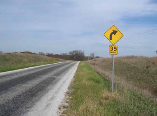
Figure 19. Horizontal curve warning sign with speed advisory plaque.
The NPA proposes the following among established engineering practices to determine the recommended advisory speed for a horizontal curve:
The ball-bank indicator readings are similar to those contained in the AASHTO Green Book (see Table 4).
Two other methods of determining a curve advisory speed have been recently outlined in a Horizontal Curve Signing Handbook prepared by the Texas Transportation Institute (19). The two methods are referred to as the direction method and the compass method. Each is discussed briefly below.
The direct method is simple to apply, requiring minimal time and cost. The first step is to record 125 or more free-flow passenger cars in each direction of travel and compute the mean speed separately for each direction. The speed measurements should be measured within the middle third of the curve. Free-flow vehicles are those with at least three seconds of space between leading and following vehicles. The second step is to multiply both average speeds from the first step by 0.97, which approximates the average truck-speed. The advisory speed for each direction is calculated by adding 1 mph to the average truck speed and then round down to the nearest 5 mph increment, unless the value ends in a 4 or 9. If the value ends in a 4 or 9, then it should be rounded up to the next 5 mph increment. This value should be confirmed by driving the curve at the advisory speed.
The compass method requires field data, which are then used as input in a truck speed prediction model. The average truck speed from the model is recommended as the advisory speed. To be accurate, the method requires that the curve length be at least 200 feet long and the curve deflection angle should be at least 15 degrees. In the first step of the procedure, the analyst must measure the curve deflection in the direction of travel, heading at the 1/3 point of the curve, ball-bank reading of curve superelevation at the 1/3 point of the curve, the length of curve between the 1/3 and 2/3 points of the curve, the heading at the 2/3 point of the curve, and the posted speed limit or 85th percentile speed on the tangents near the curve. A digital compass, distance-measuring instrument, and ball-bank indicator are required to make the field measurements. In the second step of the procedure, the Texas Curve Advisory Speed (TCAS) software is used to compute a "rounded speed advisory." This speed should be confirmed by driving the curve at the recommended advisory speed.
The intent of the compass method is to improve the process for determining curve advisory speeds – the MUTCD indicates that advisory speeds may be based on the 85th-percentile speed of free-flowing traffic, the speed determined by an engineering study, or the speed corresponding to a 16-degree ball-bank indicator reading (16). A ball-bank indicator is normally attached to a vehicle such that its physical presence will not change while driving through a horizontal curve. The ball-bank indicator reading is a function of the lateral acceleration and roll rate of a vehicle. From this, a speed at which drivers will become uncomfortable while traversing a horizontal curve can be determined. The MUTCD ball-bank indicator method assumes a constant friction threshold for all speeds, which is not necessarily applicable to highway geometric design. The compass method accounts for variable side-friction thresholds for different speeds.
Specific details concerning the direct and compass methods to set curve advisory speeds can be found in Bonneson, et al. (19), or at the following link: (http://tti.tamu.edu/documents/0-5439-P1.pdf).
Friction is needed to drive, brake and corner a vehicle. Forces are transmitted between the vehicle and road through friction at the tire-road interface. The characteristics of driving maneuvers (e.g., turning radius and speed) influence the frictional demand. The available friction is a characteristic of roadway material and vehicle tire properties. It is possible but undesirable for the demand friction to exceed available friction. Think about a car trying to stop on an ice-covered section of road.
The available friction needed for both turning and stopping decreases with increasing speed. However, as vehicle speeds increase, friction demand increases. The maximum design values for friction adequately accommodate the design speed over a wide range of conditions, including poor conditions (i.e., wet/icy pavement, worn tires, smooth road). However, at some level of speed, the available friction will be exceeded. High speeds, alone or in combination with other factors, increases the probability that available friction will be exceeded by the demand. Adverse environmental conditions (e.g., wet weather) increase the frequency of this condition and one of its more common results, skidding.
The need for friction is a major consideration in the selection and application of materials and treatments for all pavements. Many transportation agencies also have programs to increase skid-resistance at particularly vulnerable locations, such as curves and intersections. Examples of treatments used by agencies include: bituminous surface treatments, chip seals, grooving and microtexturing.
Bituminous surface treatments should include aggregate gradations that create voids in the material. This is intended to increase surface drainage as well as improve skid resistance. Agencies should first repair all major surface defects and then apply a bituminous tack coat. Finally, a bituminous surface treatment can then be overlaid onto the roadway surface. Figure 20 is an example of a bituminous surface treatment.
Figure 20. Example bituminous surface treatment.
Grooving the surface of a horizontal curve can be completed using a portable milling machine. An accepted technique is to use carbide-tipped flails to install grooves 3/16 to 3/8 inch wide and 5/32 to 5/16 inch deep, with 8 grooves per foot on a random spacing (20). Longitudinal grooves have been shown to increase directional control of the vehicle while transverse grooves are most effective at locations where vehicles are making stops.
Microtexture is the small-scale roughness that is related to the fine aggregate in a mix (21). Microtexture relates to the size of small aggregate and the surface roughness of larger aggregate. As pavement wears and weathers over time, microtexture can be lost. This can be avoided by using high-quality, skid resistant aggregate. However, microtexture loss can be restored through pavement overlays, such as open-graded friction courses. Diamond grinding Portland Cement Concrete (PCC) increases the microtexture by dislodging sand particles in the mix. The longitudinal direction of grinding also increases directional stability of vehicles.
Chip sealing is the process of sealing an asphalt roadway surface with a polymer-modified asphaltic emulsion and crushed aggregate (22). The emulsion seals the cracks in the roadway surface, keeping moisture out of the surface and base. The crushed aggregate provides for increased friction as well as an all weather wearing surface.
Speed display signs measure the speed of approaching vehicles, typically with radar, and display the measured speed. LED (light emitting diodes) is a common display technology. The signs may be mounted on trailers to increase portability or on fixed support systems. An example dynamic speed display sign is shown below in figure 21. Many of the signs also display the applicable speed limit, creating a direct comparison for drivers. Speed display signs were originally used in connection with temporary conditions, such as works zones. More recently, agencies have deployed and begun to evaluate the effectiveness of these signs in reducing speeds at permanent, speed-sensitive locations. One study (23) investigated installations at three locations and found various levels of speed-reduction effectiveness. For example, a speed display sign installed at the entry of a school zone led to a 9-mph reduction in the average speed. Smaller reductions were found at other locations.

Figure 21. Example dynamic speed display sign.
On the basis of this evaluation, the researchers offered the following insights on how various factors affect the effectiveness of speed display signs:
Speed display signs are available from a number of vendors.
Traffic calming is a term used to describe a set of techniques, consisting mostly of physical features, to affect vehicle operations on one or more streets to improve the street environment for other users (i.e., those not using motorized vehicles). Speed reduction is one of several traffic calming objectives. The specific traffic calming measures selected for application at a particular location should correspond with the unique conditions of the location and the objectives, since not every speed calming technique is appropriate for every roadway. Also, including such measures can result in drivers slowing at the speed calming feature, and speeding between them. Some of the measures that have been employed to reduce vehicle speeds include:
As noted above, traffic calming encompasses many issues other than speed management. This short summary, which emphasizes speed considerations, should not serve as the basis for traffic calming decisions. The Institute of Transportation Engineers (ITE) and the FHWA have brought together the experiences and practices of many individuals and agencies in the informational report Traffic Calming: State of the Practice (24). The report is for informational purposes and does not recommend the preferred or appropriate treatment for a particular location or set of conditions. The report includes more detailed information on the installation and reported effectiveness of specific measures and devices.
Variable speed limits are speed limits that change based on road, traffic, or weather conditions. At a particular time and place, the applicable speed limit reflects some of the same factors a prudent driver also considers. Examples include the effects of reduced visibility and slick road conditions (which may increase the required stopping distance). Improving the consistency between a responsible driver’s speed selection and the speed limit may help to restore speed limit credibility and improve safety.
The experience base with variable speed limits in the U.S. is limited. Quite a few agencies use changeable message signs to display speeds that vary with prevailing conditions but nearly all of these systems display advisory speeds. The underlying algorithms and display technologies may be very well developed but the enforcement and legal sanctions that define speed limits are not present. The most familiar U.S. application of variable speed limits is in school zones, where the speed limit changes in relation to the school schedule. Although not common, states are beginning to experiment with systems that could lead to variable speed limits in work zones.
The movement toward variable speed limits in the U.S. is in its early development phase. The legal doctrine and enabling legislation will evolve through legislative action and judicial review and interpretation.
AASHTO stopping sight distance values were revised in 2001 due to the different parameters of the changing vehicle fleet. Since the new recommended stopping sight distance values are greater than the old minimum stopping sight distance criteria (although less than the requirement for desirable stopping sight distance), this has resulted in many roadways falling outside the current range of criteria, even though the stopping sight distance design criteria was met at the time. It has been published that "moderate reductions in minimum sight distance do not appear to be a safety problem (9)." Stopping sight distance profiles can show a designer where sight restrictions occur, and the amount of sight distance that is actually available at that location. Figure 22 shows an example sight distance profile that was produced from the IHSDM.
The first mitigation measure to increase available sight distance is to lengthen crest vertical curves. This measure, however, can be quite costly and can have significant impacts to adjacent land uses. If severe sight distance limitations exist, improvements can be made even if the minimum SSD is not met. Other improvements that can be made are to remove objects that are within the sight limited area as well as increase crash avoidance areas through lane widening or shoulder widening.
The available sight distance along horizontal curves and at intersections can be improved by controlling vegetation. Vegetation can decrease the sight distance available to traffic control devices as well as decrease sight distance on the inside of horizontal curves. Another mitigation measure for inadequate sight distance on an intersection leg is to install warning flashers on the approach leg.
Figure 22. Example stopping sight distance profile from the IHSDM.
Following are some of the key points included in this Informational Guide:
Given:
Designated Design Speed = 60 mph
Radius = 716.20 ft
Superelevation Rate = 6.6 %
e(max) = 8 %
Determine the inferred design speed based on Green Book criterion for horizontal curvature based on a method 2 distribution. The method 2 distribution assumes that all lateral acceleration is first used by the friction and the rest is distributed to the superelevation rate using the following equation:
where:
e = rate of superelevation, percent;
f = side friction (demand factor);
V = vehicle speed, mph;
R = radius of curve, ft.
Rearranging the equation to solve for the inferred design speed yields:
An iterative process is used to determine the inferred design speed using the maximum friction values, maximum superelevation, and design speed from Exhibit 3-15 of the Green Book (1).
Since the maximum superelevation is not used, it is obvious that a radius that exceeds the calculated minimum will be necessary. Thus, beginning with the existing radius, existing superelevation, and a design speed of 50 mph, determine if the maximum friction of 0.14 is exceeded as follow.
f = 0.1667, which exceeds the maximum friction value of 0.14.
The next iteration is to try a 49 mph design speed with a maximum friction value of 0.142
f = 0.157, which exceeds the maximum friction value of 0.142
The next iteration is to try a 48 mph design speed with a maximum friction value of 0.144
f = 0.148, which exceeds the maximum friction value of 0.144
The next iteration is try a 47 mph design speed with a maximum friction value of 0.146
f = 0.140, which does not exceed the maximum friction value of 0.146
From this point, it can be stated that the maximum one mile-per-hour increment of speed that the existing features meet is a 47 mph design speed. Therefore, the inferred design speed for this horizontal curve is 47 mph.
An assumption that is used in this calculation is that available friction for design speed values is linear between speed increments. This assumption is true for design speeds that meet and exceed 40 mph.
Given:
A crest vertical curve has the following attributes:
g1 = +2.6%
g2 = -3.5%
Length = 800 ft
Determine the inferred design speed based on Green Book stopping sight distance criterion for a vehicle traveling from left to right.
Using terminology and criteria in the 2004 Green Book, the following are determined:
Using the Green Book recommended values for driver eye height and object height and a given L (vertical curve length) and A (algebraic difference in grades), the reduced form equations below are used to determine S (sight distance):
The first equation controls (S < L) and S = 532 ft.
The minimum stopping sight distance criteria are provided in the Green Book for design speeds in 5 mph increments. The value of 532 ft falls between the values associated with 55 mph (495 ft) and 60 mph (570 ft). The highest even 5-mph increment for which stopping sight distance is met is 55 mph. Interpolating leads to an estimate of 57.5 mph. A more precise estimate can be obtained by using the basic sight distance formula (2004 Green Book Equation 3-2) to compute the corresponding speed. This approach yields an estimate of 57.7 mph. Grades can also affect stopping distance but no adjustment is appropriate in this case. Keeping in mind the various assumptions and approximations, an estimate rounded to the nearest one mph is recommended, 58 mph in this example.
The inferred design speed can also be calculated for vertical curves if the available sight distance is known. The available sight distance can be measured through field surveys, as-built plan and profile sheets, and through existing software packages such as IHSDM.
The following equation can be used to determine the inferred design speed with the available sight distance being known:
where:
SSD = Available stopping sight distance
V = Design speed (or inferred design speed)
t = perception-reaction time (assumed to be 2.5 seconds)
a = deceleration rate (assumed to be 11.2 ft/sec2)
Given:
Crest vertical curve
Minimum SSD = 485 ft
Having put the stopping sight distance equation into a spreadsheet file, the required stopping sight distance for 0.5 mph increments can be shown as follows.
Speed (mph) |
Stopping Sight Distance (ft) |
45 |
359.739 |
45.5 |
365.920 |
46 |
372.148 |
46.5 |
378.425 |
47 |
384.750 |
47.5 |
391.122 |
48 |
397.543 |
48.5 |
404.011 |
49 |
410.528 |
49.5 |
417.093 |
50 |
423.705 |
50.5 |
430.366 |
51 |
437.075 |
51.5 |
443.831 |
52 |
450.636 |
52.5 |
457.488 |
53 |
464.389 |
53.5 |
471.337 |
54 |
478.334 |
54.5 |
485.378 |
55 |
492.471 |
55.5 |
499.611 |
56 |
506.800 |
56.5 |
514.036 |
57 |
521.321 |
57.5 |
528.653 |
58 |
536.034 |
58.5 |
543.462 |
59 |
550.939 |
59.5 |
558.463 |
60 |
566.036 |
As can be seen from this table, the available stopping sight distance does not quite meet the requirements for a 54.5 mph design speed. Rounding to the nearest mph, the inferred design speed for this curve is 54 mph.
This same method can be applied to horizontal curves that have a sight obstruction on the inside of the curve. When the available sight distance is calculated or found from field survey, the same equation can be applied for determining the inferred design speed.