U.S. Department of Transportation
Federal Highway Administration
1200 New Jersey Avenue, SE
Washington, DC 20590
202-366-4000
The need for speed management is generally determined by reviewing actual speeds and crash histories, as well as road user needs. Speed studies also assist in setting or modifying speed limits. Speed and crash information support quantifying the impact of installed countermeasures or practices. This chapter discusses speed and crash studies that are applicable to rural communities at both the transition zones and in town center areas.
Generally, a speeding or speed-related crash problem is documented before resources are committed to implementing countermeasures. Agencies should also ensure speed limits are appropriately and consistently set (and properly signed, per the guidance laid out in Chapter 2). Detailed guidance on setting appropriate speed limits is beyond the scope of this ePrimer. However, outside resources for review are provided in Section 3.4. Transition zones entering a rural community should also be properly designed. Guidance on setting appropriate transition zones is provided in Chapter 4.
3.1.1 Collecting Speed Data
The most common method to assess speeding issues is through spot speed studies. Spot speed is measured at a specific point along a roadway segment as shown in Figure 3-1. Using this method, speed is recorded at one particular location and only indicates speed at that point. When taking multiple spot speed measurements from a single location over time, and averaging them together, the resultant value is frequently referred to as "time mean speed," "mean speed," or simply, "average speed."
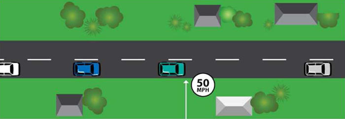
Figure 3-1 Measuring Spot Speed. (Image Source: FHWA)
A more robust method of speed measurement can be done wherein speed is measured at various points along a road segment and then averaged, as shown in Figure 3-2. This methodology is typically referred to as "space mean speed," and can provide a more complete picture of speed behavior through a corridor. An alternative method of computing space mean speed can be done by calculating speed directly using a known length of roadway, and the measured amount of time it takes a vehicle to traverse the segment.
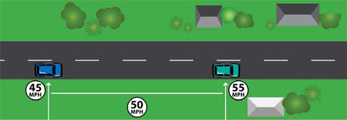
Figure 3-2 Measuring Average Speed.
(Image Source: FHWA)
Spot speeds are typically collected at problem locations to determine compliance with posted speed limits. Spot speeds can be collected using such devices as handheld radar or laser guns, pneumatic road tubes, or radar-based traffic counters. Speed can also be collected manually;detailed guidance on manual speed data collection practices has been developed by Iowa State University's Institute of Transportation (Smith, 2002).
While space mean speed can provide a more robust profile of speeding activity throughout a corridor, it is more time-consuming and difficult to collect, is a less-relatable concept by the general public, and in many cases is unnecessary, as spot speed data (when collected properly) will adequately serve to identify speeding issues. Consequently, this ePrimer will focus on using spot speed data to identify and characterize speeding problems in transition zones and rural town centers.
A spot speed study must be based on a representative sample of actual speeds. An ideal sample size is dependent on a number of factors such as observed speed variability, but various studies have suggested a minimum sample size of 50 to 125 vehicles (TxDOT, 2015; Garber and Hoel, 2002; Ewing, 1999). TxDOT (2105) provides the following guidelines for conducting speed studies:
The practitioner should also be cognizant of the fact that average speeds can vary over the course of the day. It may be advisable to collect speeds for different time periods, such as during the peak commuting periods (e.g., 7 a.m. to 9 a.m., 4 p.m. to 6 p.m.), during other peak periods for sensitive land uses (e.g., during school start/dismiss times), and at other relevant times, like day versus nighttime, depending on the issues identified and the needs of the community.
3.1.2 Identifying a Speeding Problem
Speeding is typically defined as exceeding the posted speed limit or traveling too fast for conditions. Speeding problems are identified by comparing different speed metrics against the posted speed. The most common metric is mean speed which is an average of spot speeds at the location of interest. A distribution of speeds is shown in Figure 3-3 and as noted, mean speed is between 31 and 32 mph.
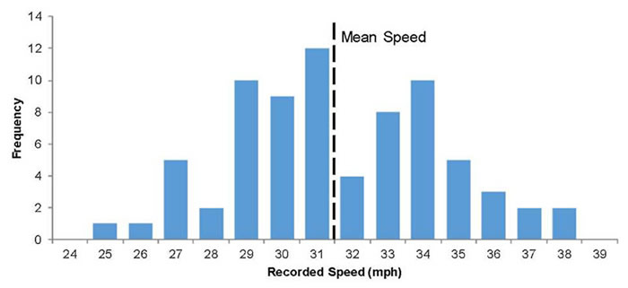
Figure 3-3 Mean Speed
The 85th percentile speed metric is also used and is defined as the speed at or below which 85 percent of vehicles travel. Figure 3-4 illustrates the 85th percentile speed using a cumulative distribution plot of the same spot speed data utilized for Figure 3-3. Here, the 85th percentile speed is approximately 34.5 mph compared to the mean speed of 31.5 mph. In this scenario, 85 percent of drivers were traveling 34.5 mph or lower.
Some studies have used the number of drivers exceeding a particular speed threshold (Hallmark et al., 2007). This metric is the number of drivers who are traveling a specific amount over the posted speed limit. For example, 22 percent of vehicles are 20 or more mph over the speed limit. Vehicles exceeding a particular threshold is a measure of excessive speeding.
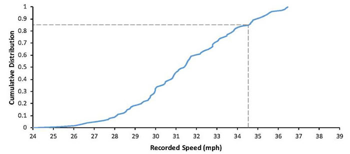
Figure 3-4 85th Percentile Speed
A typical metric for establishing a speeding problem is a mean speed of 5 or more miles per hour (mph) over the posted speed limit (VDOT, 2008). Other agencies consider an 85th percentile speed which is 7 to 10 mph over the posted speed limit as a speeding issue. Some agencies suggest a volume threshold (e.g., more than 1,000 vehicles per day) as well as a speed threshold (PennDOT, 2012) before speed management and speeding countermeasures can be considered.
Identifying a speeding problem assumes existing speed limits are reasonable and prudent for the prevailing roadway design, traffic, and environmental conditions. In situations where roadway characteristics, traffic patterns (e.g., volume, fleet mix, commuting trends), or land use (e.g., development type, access points) have changed, posted speed limits should be reviewed. However, it must be emphasized that lowering speed limits alone does not necessarily encourage drivers to slow down, and should not be relied upon as an effective speed management strategy.
Traveling too fast for conditions is also commonly used to define a speeding problem (Liu and Chen, 2009). This definition entails drivers exceeding a reasonable speed given prevailing roadway or traffic conditions. A so-called "reasonable speed" could be less than the posted speed limit, depending on environmental conditions. Wet, icy, or snowy roadway surface conditions may result in decreased friction, which increases stopping distance, and necessitates lower driving speeds. Additionally, under certain weather conditions such as rain or snow, reduced visibility may impact sight distance, further increasing the risk to all roadway users of maintain the posted speed limit. Highly-congested or irregular traffic conditions may also call for decreased speeds. For instance, in many rural communities, during spring planting or fall harvesting, the presence of oversized and slow-moving vehicles may dictate lower travel speeds so that drivers encountering these vehicles are able to react appropriately.
3.1.3 Speed Analysis
Comparison of speed metrics (e.g., mean speed, 85th percentile speeds, or percent traveling over a certain speed threshold) before and after installation of a speeding countermeasure is commonly used to assess the effectiveness of the countermeasure. Speeds can be compared at the treatment location as well as some distance upstream or downstream on the roadway. It is important to note that frequently, traffic patterns and driver behavior will change immediately after installation of countermeasures, but may revert to previous patterns as drivers acclimate to the treatment. For this reason, monitoring of speeds for 6 months to 1 year is suggested to reduce the influence of this altered behavior on countermeasure effectiveness assessment (PennDOT, 2012; VAT, 2003). An example of assessing change in speed due to the use of speeding countermeasures is provided in the example below.
Example 3-1: Speed Analysis
The community of Slater, Iowa (population 1,306) was identified as having speeding problems near the community entrances. The speed limit at the south community entrance is 25 mph. Spot speeds were measured with a mean speed of 32 mph and 85th percentile speed of 36 mph.
Tubular channelizers were placed as shown in Figure 3-5. Speeds were measured again after the treatment had been in place for 1 month.
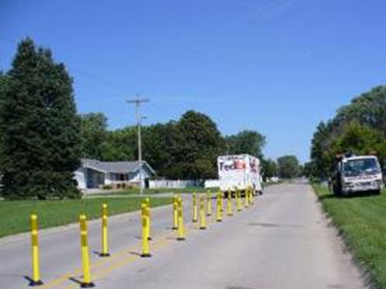
Figure 3-5 Treatment in Slater, Iowa. (Image Source: Neal Hawkins)
Mean speeds decreased by 5mph, from 32mph to 27mph, with the installation of the channelizers, as shown in Figure 3-6.
The 85th percentile speed also decreased by 3mph, from 36 mph to 33 mph.
Additionally, the fraction of vehicles traveling over the speed limit by 5 and 10 mph thresholds were compared (see Table 3-1).
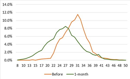
Figure 3-6 Comparison of Speed Metrics
Before the countermeasure installation, 689 of 2929 vehicles (23.5 percent) were traveling 10mph or more over the posted speed limit of 25mph. At one month after installation, 281 of 2553 (11.0 percent) were traveling at that speed. Simillarly, 5.3 percent of vehicles were traveling 15mph or more over the posted speed limit before the countermeasure installation and 2.3 percent were at that threshold after installation.
Table 3-1 Comparison of Vehicles Traveling Set Amount over Speed Limit
| Speed Threshold | Before | After (1-month) | ||||
|---|---|---|---|---|---|---|
| Total Vehicles | Vehicles Exceeding Threshold | % Exceeding Threshold | Total Vehicles | Vehicles Exceeding Threshold | % Exceeding Threshold | |
| > 35mph | 2929 | 689 | 23.5% | 2553 | 281 | 11.0% |
| > 40mph | 2928 | 154 | 5.3% | 2552 | 58 | 2.3% |
A measurement of crashes on the roadway is the best indicator of safety. However, crashes are generally infrequent and random events in rural areas. As a result, it may be difficult to detect a crash problem at a particular location, with only a few years of data available to the practitioner.
3.2.1 Collection of Crash Data
Crash analyses typically require the following data:
Data are typically collected along a study segment where a problem is suspected. Since crashes are random events, they can fluctuate over time. As a result, several years of data should be evaluated so that short term anomalies do not drive the analysis. In many cases, a minimum3 to 5years of data are used to determine a crash problem, or to assess a change in crashes after installation of a countermeasure. Five years is preferred when available.
Most State DOTs collect and archive crash data. Counties and cities may also collect this type of data, or have access to the State DOT crash database through a partnership or cooperative agreement. As a result, it is important crash data requests be directed to the appropriate agency. Each jurisdiction has its own criteria for which crash characteristics are collected, but the following information is normally recorded and is helpful in assessing speeding problems.
Table 3-2 Crash Variables for Speed-Related Crash Analyses
| Data Element | Description | Use | Caution |
|---|---|---|---|
| severity |
|
|
|
| speeding-related |
|
|
|
| contributing circumstance or major cause |
|
|
|
| vehicles |
|
|
|
| time of day |
|
|
|
Citizen complaints, reports from maintenance personnel, or police feedback can also be evaluated since they may be aware of near misses or minor collisions that are not reported in crash databases (Golembiewski and Chandler, 2011). Since this information is anecdotal, it is difficult to include in a formal crash analysis but this information can point to a potential safety issue particularly in rural areas where crashes are rare.
3.2.2 Crash Analysis
Determining whether a legitimate crash problem, and more specifically, a speeding-related crash problem, exists within a transition zone or a town center can be a challenge, depending on the amount of data and staff time/expertise available. For preliminary problem identification, a crash problem can be determined by comparing crash frequency, crash rate, or type of crash. While these types of techniques, detailed below, are useful as a starting point for crash analysis, more comprehensive and robust data-driven methods should be relied upon for a final determination whenever possible. Such methods, which are assembled through such resource portals as the FHWA Road Safety Data Toolbox and the FHWA Data Driven Safety Analysis Website, are beyond detailed description in this ePrimer, but represent the best practices when it comes to empirical crash analysis.
Crash frequency, also known as observed crash frequency by such prevailing literature as the Highway Safety Manual, is a measure of the historic crash data on a roadway facility (i.e., the number of recorded crashes in a given period). A local practitioner can determine crash frequency using information compiled from the State crash database or law enforcement crash reports. This will allow the practitioner to do the following:
Once crash frequency information is collected and displayed, the practitioner can complete a methodical analysis by roadway, city, or county or use techniques such as cluster analysis to determine those roadway locations that have experienced a high or moderate number of speed-related crashes. Multiple crashes at the same location may be an indication of a safety problem (FHWA, 2010; Bagdade et al., 2012). These clusters of crashes can be identified using a simple "push pin" map, as shown in Figure 3-7.
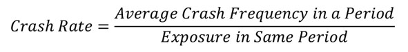
According to the Highway Safety Manual published by the American Association of State Highway and Transportation Officials (AASHTO, 2010) crash rate is the number of crashes that occur at a given site during a certain time period in relation to a particular measure of exposure (e.g., per million vehicle miles traveled). Generally, a crash rate can be computed using the following equation :
The Highway Safety Manual provides several different means of estimating crash rate, including as the annual number of crashes per million vehicle miles traveled and the number of crashes per mile per year. Many practitioners, however, are already familiar with the crashes per million vehicle miles traveled measure, which will be the focus of discussion within this ePrimer.
Crash rate analysis can be a useful tool to determine how a specific roadway or segment compares to an average roadway on the network. Crash frequency does not account for differences in traffic volume and is often inadequate when comparing multiple roadways of varying lengths and/or traffic volume.
For example, it is possible that two roadways crossing a community (Route A and Route B) each have the same number of crashes. However, Route A could have more than double the number of vehicles on a typical day than does Route B. To effectively compare the relative safety of the two locations, the practitioner must factor in the level of exposure (e.g., vehicle miles traveled) on each route.
One limitation of crash rates for low-volume roads is the sensitivity of the formula to traffic volume. The crash rate calculation is not as beneficial at low volumes as it is with higher-volume roads, as small changes in the number of vehicles results in a disproportionate change in the crash rate for the segments that, in reality, operate similarly.
Where traffic volume data is unavailable, other information can be used to provide exposure estimates. One often-used factor is the length of the roadway segment on each route studied. Comparing the number of speed-related crashes per mile can help an agency identify potential opportunities to improve safety.
Crash rate (crashes per million vehicle-miles traveled, or cpmvm) is calculated using the following formula:
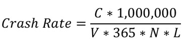
Where:
C = observed crash frequency in the study period
N = length of the study period (in years)
V = traffic volumes using AADT
L = length of the roadway segment in miles
Crash rate for the segment of interest is then compared against similar roadway segments. A more detailed example of how different crash metrics are calculated is illustrated below.
Note, that beyond basic crash frequency and crash rate analysis, there are more advanced methods of analyzing crash data, such as statistical methodologies based on Empirical Bayes, which combine a weighted average of crash data from the site of interest with crash metrics from similar sites to compute an adjusted crash risk and forecast. Practitioners should also be mindful of regression-to-the-mean phenomena, wherein short-term spikes or drops in crash frequency or crash rates could result in erroneous conclusions being drawn about the safety of a roadway segment. Regression-to-the-mean can also result in the effectiveness of speeding countermeasures being over- or understated, if a very short analysis window is used.
A detailed description of these issues and advanced methodologies is beyond the scope of this ePrimer and is outside the staff expertise of many rural transportation agencies. However, many of the analysis concerns and caveats are alleviated or eliminated by collecting crash data over longer time periods (e.g., 5 years or more). A good comprehensive resource for practitioners wanting to learn more about crash data analyses best practices, including network screening methods, is the Highway Safety Manual.
Example 3-2: Crash Analysis Calculations
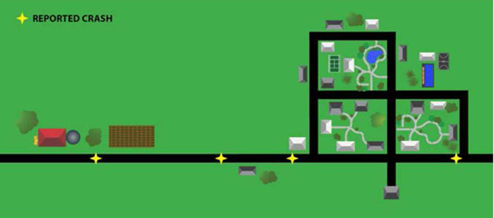
Figure 3-7 Observed crash locations. (Image Source: FHWA)
Figure 3-7 shows locations of observed/reported crashes around the community of Dunshire over a 3year period. Using the crash frequency method, it is noted that four crashes occurred within the study area. Using the crash clustering approach, three crashes are clustered near the west community entrance. Two of the crashes were coded as "Speed-related.. The pattern may suggest drivers are unprepared for the changing roadway conditions. Additionally, there is a school located within this area that raises concern for pedestrian and bicyclist safety.
The AADT along the one-mile segment of east-west main street in the study area is 1,000 vehicles per day (vpd). The Crash rate for this road segment is thus computed as:
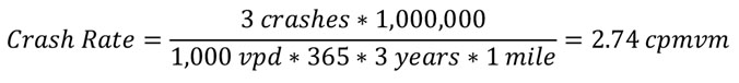
With the calculated crash rate along Main Street of 2.74 crashes per million vehicle miles, the county engineer can now contrast this with the main street crash rates of several nearby communities, which average to 2.23 cpmvm. The higher crash rate in Dunshire, along with the speed-related nature of three of crashes, and proximity to a school are all significant indicators that a speeding issue may exist on the roadway heading into the community.
Rural corridors often serve as the Main Street within small communities, and as the land uses transition from rural to town, so does the heightened need for motorist speed compliance. Community land uses include homes, schools, swimming pools, parks, and playgrounds, all of which generate traffic along and across the Main Street by a wide range of users from small children to the elderly, and modes such as vehicles, pedestrians, and bicyclists. In many cases, these users' sense of roadway purpose is strikingly different than that of the pass-through commuter traffic, who only travels through town twice a day and where the majority of the drive from origin to destination is at much higher speeds on roadways outside of the community. This contrast in perspectives heightens the need for speed management within our rural communities and support in balancing both mobility and safety. The practitioner should be mindful of the needs for all users, regardless of mode, they enjoy a safe, accessible, and equitable travel space, and should strive to create a roadway environment that maximizes user mobility, but not at the cost of increased crash fatalities or injuries.
3.4.1 Handbook of Simplified Practice for Traffic Studies
Source: www.ctre.iastate.edu/pubs/traffichandbook
Year: November 2002
Publisher: Institute for Transportation at Iowa State University, Ames, Iowa Description: The handbook provides a layperson's guide to traffic studies which include:
Each study includes step-by-step instructions, real-world examples, and a template project work order.
3.4.2 Roadway Safety Data Toolbox
Source: https://safety.fhwa.dot.gov/rsdp/toolbox-home.aspx
Year: 2017
Publisher: Federal Highway Administration
Description: The Roadway Safety Data Toolbox, and the associated Roadway Safety Data Portal, provides practitioners with a comprehensive access to state-of-the-art tools utilized in crash analysis and speeding-related crash problem identification. The toolbox contains multiple sections, centered around crash data collection, crash data management, and crash data analysis. There is also a section on cutting edge resources and future research needs. While many of these tools and techniques are applicable to the rural community transportation professional, some may rely on data sets and/or resources that are not accessible by smaller transportation agencies.
3.4.3 Every Day Counts, Round 4: Data-Drive Safety Analysis Resource Page
Source: https://www.fhwa.dot.gov/innovation/everydaycounts/edc 4/ddsa.cfm
Year: 2017
Publisher: Federal Highway Administration
Description: Traditional crash and roadway analysis methods mostly rely on subjective or limited quantitative measures of safety performance. This makes it difficult to calculate safety impacts alongside other criteria when planning projects. Data-driven safety analysis employs newer, evidence-based models that provide state and local agencies with the means to quantify safety impacts similar to the way they do other impacts such as environmental effects, traffic operations and pavement life.
The analyses provide scientifically sound, data-driven approaches to identifying high-risk roadway features and executing the most beneficial projects with limited resources to achieve fewer fatal and serious injury crashes. Through round four of Every Day Counts , this effort focuses on both predictive and systemic analyses—two types of data-driven approaches that state and local agencies can implement individually or in combination.
3.4.4 Improving Safety on Rural Local and Tribal Roads Safety Toolkit
Source: https://safety.fhwa.dot.gov/local rural/training/fhwasa14072/
Year: August 2014
Publisher: Federal Highway Administration
Description: The Safety Toolkit provides a step-by-step process to assist local agency and Tribal practitioners in completing traffic safety analyses, identify safety issues, countermeasures to address them, and an implementation process. Each step in the Toolkit contains a set of tools, examples, and links to resources appropriate to the needs of safety practitioners. The report presents a seven-step safety analysis process based on a similar process developed in the Highway Safety Manual. The seven steps are: compile data; conduct network screening; select sites for investigation; diagnose site conditions and identify countermeasures; prioritize countermeasures for implementation; implement countermeasures; and evaluate effectiveness of implemented countermeasures. There are two accompanying User Guides which present step-by-step processes of example scenarios.
3.4.5 Improving Safety on Rural Local and Tribal Roads Safety Toolkit - Site Safety Analysis -User Guide #1
Source: https://safety.fhwa.dot.gov/local rural/training/fhwasa14073/
Year: August 2014
Publisher: Federal Highway Administration
Description: The Site Safety Analysis (User Guide #1) demonstrates the step-by-step safety analysis process presented in Improving Safety on Rural Local and Tribal Roads - Safety Toolkit. This report specifically addresses how to study crash conditions at a curve on a rural roadway. The User Guide provides example applications of five Toolkit steps: compile data; diagnose site conditions and identify countermeasures; prioritize countermeasures for implementation; implement countermeasures; and evaluate effectiveness of implemented countermeasures.
3.4.6 Improving Safety on Rural Local and Tribal Roads Safety Toolkit - Network Safety Analysis - User Guide #2
Source: https://safety.fhwa.dot.gov/local rural/training/fhwasa14074/
Year: August 2014
Publisher: Federal Highway Administration
Description: The Network Safety Analysis (User Guide #2) presents an example scenario and step-by-step solution for studying safety conditions and identifying potential treatments at unsignalized intersections on a network. This User Guide demonstrates how to conduct network screening, select sites for further investigation, conduct safety diagnosis, select countermeasures, and prioritize and implement improvements. The User Guide provides example applications of all seven steps in the Improving Safety on Rural Local and Tribal Roads - Safety Toolkit (FHWA-SA-14-072): compile data; conduct network screening; select sites for investigation; diagnose site conditions and identify countermeasures; prioritize countermeasures for implementation; implement countermeasures; and evaluate effectiveness of implemented countermeasures.
Bagdade, J., D. Nabors, H. McGee, R. Miller, and R. Retting (November 2012). Speed Management: A Manual for Local Rural Road Owners. FHWA Office of Safety. FHWA-SA-12-027.
Golembiewski, G.A. and B. Chandler (January 2011). Intersection Safety: A Manual for Local Rural Road Owners. Federal Highway Administration, Office of Safety. FHWA-SA-11.08.
FHWA. Roadway Safety Information Analysis: A Manual for Local Rural Road Owners. Federal Highway Administration, Office of Safety. December 2010. https://safety.fhwa.dot.gov/local_rural/training/fhwasaxx1210/index.cfm
Garber. N. and L. Hoel (2015). Highway Engineering. 5th Edition. Cengage Learning, Stamford, CT.
Ewing, R. (1999) Traffic Calming: State of the Practice. Institute of Transportation Engineers. Washington, D.C.
Hallmark, S.L., E. Peterson, E. Fitzsimmons, N. Hawkins, J. Resler, and T. Welch (October 2007). Evaluation of Gateway and Low-Cost Traffic-Calming Treatments for Major Routes in RuralCommunities. Iowa Highway Research Board. www.intrans.iastate.edu/research/projects/detail/7projectID-226410767
Liu, Cejun and Chou-Lin Chen (February 2009). An Analysis of Speeding-Related Crashes: Definitions and Effects of Road Environments. National Highway Transportation Safety Administration, US Department of Transportation. DOT HS 811 090.
PennDOT (July 2012). Pennsylvania's Traffic Calming Handbook. Pennsylvania Department of Transportation. Pub 383.
Smith, D. Handbook of Simplified Practice for Traffic Studies. (November 2002). Institute for
Transportation, Iowa State University, Ames, Iowa. http://www.ctre.iastate.edu/pubs/traffichandbook
TxDOT. Procedures for Establishing Speed Zones. (August 2015). Texas Department of Transportation.
VDOT. Traffic Calming Guide for Local Residential Streets. (October 2002, revised July 2008).Virginia Department of Transportation, Traffic Engineering Division. Richmond, Virginia.
VAT. Traffic Calming Study and Approval Process for State Highways. (September 2003). Vermont Agency of Transportation. http://vtransplanning.vermont.gov/sites/aot_policy/files/documents/planning/TrafficCalming.pdf
| << Module 2 | Rural Transition Zones ePrimer | Module 4 >> |

