U.S. Department of Transportation
Federal Highway Administration
1200 New Jersey Avenue, SE
Washington, DC 20590
202-366-4000
| < Previous | Table of Contents | Next > |
Step 2 in the scalable risk assessment process is to select the geographic scale at which risk and exposure values are desired. The desired geographic scale is based on, and sometimes dictated by, the use(s) of the risk values as defined in Step 1.
The desired geographic scale for exposure estimates is an important parameter that will be used in several subsequent steps. For example, selection of exposure measures (Step 4) are informed by the desired geographic scale (i.e., certain exposure measures are better suited to detailed geographic scale, whereas other exposure measures are better suited to an areawide geographic scale). Similarly, the selection of analytic methods to estimate exposure (Step 5) are also based on the desired geographic scale. These steps later in the guide provide more detail on how scale informs these decisions.
The scalable risk assessment process includes four geographic scale categories, listed in Table 6 and shown graphically in Figure 5 in order of most granular to most aggregate. Note that the four scale categories can be grouped into two general scale groups: 1) facility-specific; and 2) areawide. These two scale groups typically use fundamentally different analytic methods to estimate exposure. This is discussed further in Step 5.
| Scale Group | Scale Category | Description | Examples |
|---|---|---|---|
| Facility-Specific | Point | Specific location where conflicting traffic streams cross, merge, or diverge. |
|
| Segment | Length of street or roadway between two points. Traffic volumes and physical characteristics generally remain the same along the length of a segment, although small variations may occur. |
|
|
| Areawide | Network | A mid-sized geographic area that includes an interconnected set of transportation facilities. |
|
| Regional | A large geographic area that includes all transportation facilities within a defined political boundary. Because of the large geographic size, land use at this scale can be heterogeneous within a defined area. |
|
Facility-Specific Scales

Areawide Scales
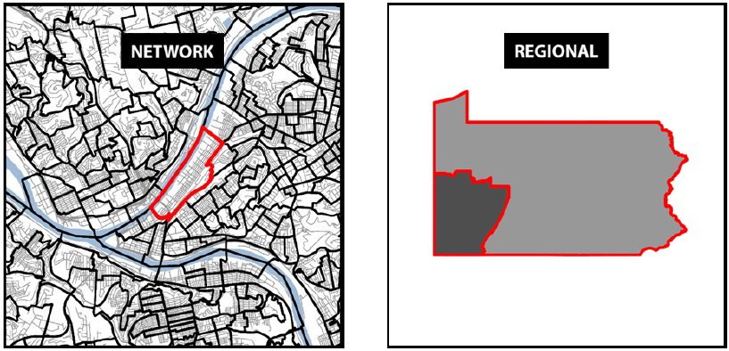
Figure 5. Illustration of Geographic Scales for Exposure Estimation
When selecting a geographic scale for risk assessment, one should consider several practicalities and limitations:
Small or zero numbers: Granular scales may be susceptible to the small numbers problem, wherein the number of crashes or exposure may be very small or even zero for some locations or areas. These small or zero values for crashes or exposure can provide results that are misleading or not useful. Caution should be used in selecting scales that are too granular for the input data.
Applying areawide characteristics to specific facilities: For facility-specific scales, some context characteristics can be derived from the encompassing area. For example, demographic or socioeconomic variables from census tracts or block groups can be applied to specific intersections or street segments within that geography. This assignment assumes that these variables are relatively constant within the defined area or geography. The assignment of area characteristics to a street segment can become more complicated if the defined segment traverses multiple areas with different characteristics. In these cases, a weighted average (based on portion of overall segment length) can be used, but one should note that these weighted averages for long segments could mask interesting contextual differences at a given location.
Major streets on defined area boundaries: Major streets and roads often form the boundaries for defined areas (such as census geographies or TAZs). Depending on the locational precision of reported crashes and street geometry, pedestrian and bicyclist crashes that occur on major streets could be split between the defined areas on either side of the major street, thereby diluting the number of crashes that are assigned to each area on either side. In turn, this could lower the calculated crash frequency and risk values for these areas where a major street forms a boundary, providing misleading results for both areas.
In some cases, several geographic scales may be desired for the exposure and risk values. For example, one may want to develop risk values at the segment level as well as for TAZs. In cases when multiple geographic scales are desired, one should select the most granular desired scale for estimating exposure and risk, and the more aggregate desired scales can be calculated by combining the granular exposure estimates (assuming that the more granular exposure estimates are feasible to calculate). Later sections in this chapter discuss this aggregation process in more detail. Note that it is much less feasible to estimate exposure at an aggregate scale and then decompose the aggregate values to a more granular scale.
As shown in the rightmost column of Table 6, there are multiple possible scales within each of the four scale categories. For example, the Segment scale category could include several possible scenarios such as short segments between intersections, longer segments that traverse multiple intersections, or even multiple parallel segments in a miles-long corridor. However, in all of these possible scenarios, the exposure will be estimated at its base scale unit (in this case, a segment), and then aggregated up to the desired analysis, reporting or presentation level. The following sections provide several examples of aggregating to slightly different scales within the same scale category (as shown in Table 6).
Figure 6 illustrates that multiple crosswalks can be aggregated up to the intersection point (I) by summing the total crossings per crosswalk (A+B+C+D) (Radwan et al. 2016). Pedestrians or bicyclists that turn a corner on the sidewalk without crossing the street are not counted since they did not enter a shared space with motor vehicle traffic. Each crosswalk is treated as a separate location with its own crossing count, thereby capturing the number of times a pedestrian or cyclist is exposed to motor vehicle traffic.
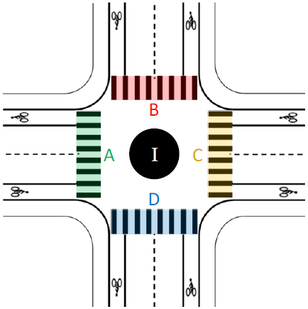
Figure 6. Illustration of Combining Individual Crosswalks for Intersection Exposure
Two-way segment-level volume data can be used to estimate intersection volume if dedicated intersection count data do not exist (Wang et al. 2016). As shown in Figure 7, each leg of an intersection (A, B, C, D) represented by individual segments and should be summed and then divided by two to equal the total intersection volume represented as a point (I). Depending on the segment-level volume data, this method may exclude specific types of traffic, such as pedestrian traffic on sidewalks that does not cross a street at the designated intersection.
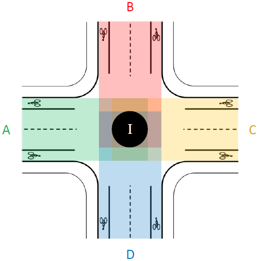
Figure 7. Illustration of Estimating Intersection Exposure from Segment Counts
Corridor volumes can be calculated by aggregating the volume multiplied by length for each of the parallel segments that make up the corridor, e.g. roadways, bikeways, multi-purpose paths, etc. The example below shows the Cesar Chavez Blvd. corridor in downtown Austin, Texas along Lady Bird Lake, which is comprised of a roadway, a multi-purpose path, and a bikeway, as shown in Figure 8.
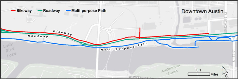
Figure 8. Illustration of Multiple Parallel Facilities in a Corridor
Figure 9 shows each facility divided into segments with dots as segment endpoints. In this example, bicycle-miles of travel (BMT) is calculated using crowd-sourced data as bicycle counts for each of the facility segments and then summed to equal the total BMT for per facility in the corridor. Table 7 shows the BMT totals per facility, which were summed to equal the total BMT for the entire corridor.
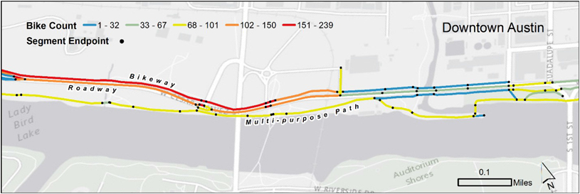
Figure 9. Illustration Showing Count Segments on Multiple Parallel Facilities in a Corridor
| Facility | Number of Segments | BMT |
|---|---|---|
| Bikeway | 14 | 183 |
| Roadway | 24 | 148 |
| Multi-purpose Path | 33 | 149 |
| Corridor Total | 71 | 480 |
Figure 10 illustrates how smaller individual street segments could be combined into a longer segment. The example is for University Drive in College Station, Texas that runs along a major university, of which Wellborn Road bisects into Central Campus and West Campus districts. Each district has its own unique urban character that could possibly affect pedestrian traffic, and therefore, the roadway is treated as separate segments. In this case, pedestrian-miles of travel (PMT) would be calculated per roadway segment in each district and summed to equal total PMT for a both West Campus and Central Campus University Drive.

Figure 10. Illustration of Multiple Segments Being Combined into Single Longer Segment
The example below (Figure 11) shows the region, represented by Travis County, Texas, subdivided by Census tracts to represent a network level scale. Each tract contains the average daily BMT, which can be summed to total the regional average daily BMT.
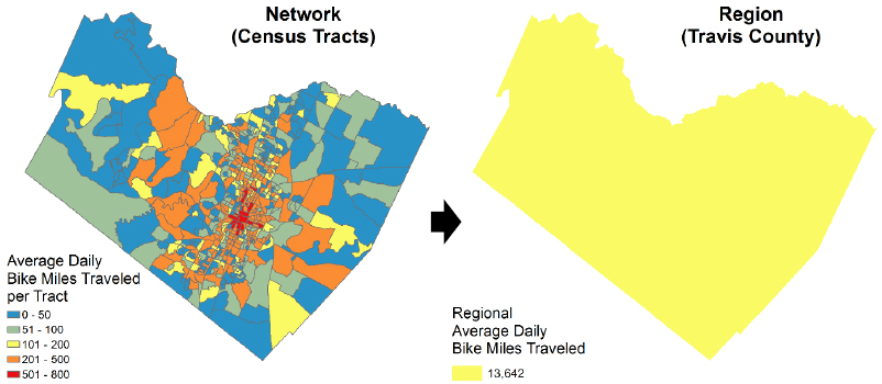
Figure 11. Illustration of Multiple Census Tracts Being Combined into Single Region
| < Previous | Table of Contents | Next > |

