5.0 Using Safety Analyses for Planning

For many transportation planning organizations, the biggest barrier to integrating quantitative safety analysis into the planning process is staff time and expertise. While this can be a significant barrier, agencies can begin to address safety with a low level of effort. First and foremost, planners should coordinate with data managers in their States to learn about data availability, analyses already complete, and/or options for analytical support specific to the planning jurisdiction. For example, the State SHSP may include data analysis and/or safety emphasis areas that are relevant to the planning agency. Funding for transportation safety analysis, research, and/or project implementation may be available through the State DOT HSIP; or the State TRCC may have resources available for data collection, analysis, or evaluation projects.

Another way to overcome these barriers is to start small. Many of the analyses using descriptive statistics can be conducted using common spreadsheet tools. Summarizing the who, what, when, where, and why of crashes will provide an excellent starting point to understanding safety conditions in the community. This information can serve as talking points to elected officials and local partners and raise the importance of safety in the community.

This section provides an overview of the basic safety analysis categories, questions answered in each category, how this can be included in transportation planning, and analysis methods to answer these questions. The topics covered are presented in table 5.1. This guidebook focuses on basic analysis methods. As data, expertise, resources, and interest grows, more advanced methods should be considered. A more detailed version of table 5.1, including methods, data needs and tools is included in appendix B.

Table 5.1 Safety Analysis Categories and Questions

Analysis Category	Analysis Question
Benchmarking	How many fatalities and serious injuries are occurring in my area? How does this compare to other areas or my State?
Identify Crash Trends and Contributing Factors	Who is involved in crashes? When are the crashes occurring? What are the major contributing factors to crashes?
Identify and Evaluate Focus Crash Types	What are the most common crash types? What are the most common contributing factors? What are the characteristics of the over representation?
Network Screening—Identify Sites for Safety Improvement	What locations (intersections or segments) show the most potential for safety improvements?
Systemic Analysis—Identify Safety Risk Factors	What are the common characteristics of locations with crashes? What are the countermeasures to address these characteristics? How should we prioritize systemwide implementation?
Corridor and Intersection Planning Safety Analysis	What are the safety effects of alternative roadway or intersection cross sections?

5.1 Benchmarking

Integrating safety analysis into planning- and project-level activities starts with understanding the scope and scale of safety concerns in the planning area. Initially, planners need to understand performance measures such as: number of fatalities; number of serious injuries; rate of fatalities; and rate of serious injuries.

Benchmarking the area’s safety performance for a particular period is useful in the long-range planning process as part of setting plan vision and goals and establishing performance measures and evaluation criteria for the plan. Fundamentally, benchmarking like this makes it possible to monitor safety performance within the area, as well as assess performance of the system relative to other comparable areas and/or the State. At the highest level, these performance measures quantify the number of people killed or seriously injured over time in the area. Monitored annually, this will provide the agency with information about overall effectiveness and safety planning and programming in the area and will help transportation agencies determine the appropriate safety focus areas moving forward.

5.1.1 Methods for Benchmarking

In descriptive analyses for benchmarking, areawide crash frequency and crash severity per year are tallied for a period of years to develop a simple trend summary. This trend can be summarized for the area only to evaluate current performance to past years, or performance in a specific year can be compared to similar data from other areas to compare performance across areas. Figure 5.1 shows annual total crash fatalities and serious injuries for a community for the years 2009 to 2013. Figure 5.2 shows a comparison of fatalities by DOT region.

Figure 5.1 Chart. Fatalities and Serious Injuries per Year

Source: Sample data, Cambridge Systematics, Inc., 2015.

Figure 5.2 Chart. Comparison of Fatalities by Region

Source: Sample data, Cambridge Systematics, Inc., 2015.

5.2 Identify Crash Trends and Contributing Factors

The next category of safety analysis is conducted to identify major crash trends and contributing factors in a community. The crash trends and contributing factors tell the safety “story” of who, what, when, where, and why people are involved or injured in crashes:

• Who? Age distribution and gender of crash victims.
• What? Number and type of vehicles (single or multivehicle crashes, commercial vehicles or passenger vehicles), pedestrians, motorcyclists, bicyclists, etc., involved in the crash.
• When? Year, month, day, and hours of crashes.
• Where? Crash location by roadway functional classification, intersection or roadway segment, urban or rural environment, transportation analysis zone, or subdistrict within the community.
• Why? Behavioral and environmental factors, such as driver impairment, driver distraction, speeding, pavement condition, or road curvature.

The objective of this analysis is to understand the major safety trends in a community and identify if there are crash types or contributing factors that are more common than expected; and, as a result, should be a focus of project planning, policy or programming, and prioritization. Analyses like these can be conducted for safety-specific plans, or can be conducted as part of an existing conditions assessment in a long-range or corridor plan. Knowing crash trends and contributing factors can help transportation agencies determine appropriate safety countermeasures during these planning processes.

5.2.1 Methods for Identifying Crash Trends and Contributing Factors

Descriptive statistics count and compare the number (i.e., frequency), type, severity of crashes, and/or contributing factors that have occurred historically. Typically, this is done for the most recent three- to five-year period at a site, along a corridor or in an area. As described in the bullets above, there are many possible contributing factors and categories to count. As such, it is advisable to start with a small number of categories to keep the process manageable. As specific concerns arise within any given category, it may be necessary to dig deeper into the data.

Figures 5.3 through 5.6 show example analyses. Figure 5.3 shows for a one-year period, the percentage of all crashes occurring during each hour of a day and the percent of severe crashes by hour of day. As shown, in this data set, the greatest percentage of severe crashes is occurring between noon and 1:00 p.m. Considering all crashes, 3:00 to 4:00 p.m. is the most common period for crashes.

Figure 5.3 Chart. Distribution of Total and Severe Injury Crashes, by Time of Day

Source: Sample data, Cambridge Systematics, Inc., 2015.

Figures 5.4 through 5.6 show crash distribution by age and gender. In this data set, 25- to 34-year-olds have the most crashes, severe and total. This figure also shows that approximately half of all crashes and nearly two-thirds of all severe injury crashes involve a male.

Figure 5.4 Chart. Distribution of Total and Severe Injury Crashes by Age

Source: Sample data, Cambridge Systematics, Inc., 2015.

5.3 Identify and Evaluate Focus Crash Types

With an understanding of the major crash trends and contributing factors, the planning agency may select one or more of the more prominent crash trends or contributing factors as a focus for planning and programming activities. For example, the crash trend assessment may show more pedestrian or bicycle crashes than expected for a particular area of the community. As a result, a pedestrian/bicycle safety action plan could be developed for the particular area, or the community may find roadway departure crashes in the rural part of the community are overrepresented. In this analysis, the planner would review and summarize crash data to understand such topics as:

• What is the manner of collision? Rear-end, angle, roadway departure, head-on? Was a pedestrian or bicycle involved?
• What is the crash severity? Which crash types are most severe and where are they occurring?
• What crash types or contributing factors are overrepresented?
• What is the geographic distribution of the focus crash type?
• What are common roadway features?

As an outcome of this analysis, the transportation planner would understand the categories of crashes by type, severity, contributing factor, or geography that may be a focus for planning, programming, and countermeasure identification; or the types of crashes or contributing factors that should be a consideration in non-safety-specific projects.

For example, figure 5.7 considers crash distribution by Transportation Analysis Zone (TAZ). The figure shows the percentage of roadway departure crashes per TAZ as a total of all crashes in each TAZ. As shown, roadway departure crashes are more common on the east side of the region, particularly in the southeast.

Figure 5.7 Map. Distribution of Roadway Departure Crashes by Transportation Analysis Zone

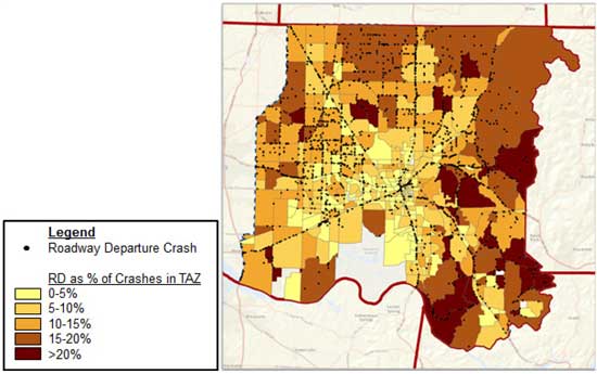
Source: Cambridge Systematics, Inc., unpublished, prepared for Alabama Department of Transportation.

5.3.1 Methods for Identifying and Evaluating Focus Crash Types

Scatterplot

The scatterplot (figure 5.8) illustrates a simple method for evaluating the relative occurrence of various crash types in terms of frequency and severity. The x-axis represents the crash type frequency rank, while the y-axis indicates the crash type severity rank (percentage of crashes that result in a severe injury). In this example, the single-vehicle (RD) crash type stands out as being highly ranked in both frequency and severity. At the other extreme, backing and other crashes are ranked in the bottom in both frequency and severity and, therefore, are relatively unimportant. Depending on the interest of the MPO, greater emphasis could be placed on frequency or severity.

Figure 5.8 Scatterplot. Crash Types by Frequency and Severity Ranking

Source: Sample Data, Cambridge Systematics, Inc., 2015.

Overrepresentation

Overrepresentation is another measure of whether a crash type or contributing factor should be prioritized as a safety issue in the planning area. One way to visualize overrepresentation is to compare the percentage of all crashes accounted for by a given factor with the percentage of severe crashes (those resulting in a fatal or serious injury) accounted for by that same factor. For example, figure 5.9 shows 15 percent of all crashes are single vehicle roadway departure crashes, yet 33 percent of all severe crashes are roadway departure crashes.

Figure 5.9 Chart. Overrepresentation of Severe Crashes among Select Crash Types

Source: Sample Data, Cambridge Systematics, Inc., 2015.

Risk Ratio

Another method for identifying if a particular crash type, contributing factor, or severity should be considered as a focus for the area is called risk ratio. The risk ratio compares the severity of crashes associated with a particular factor to the severity of all other crashes. Using the risk ratio analysis method shown in appendix C, it is possible to learn if a particular crash type in a given situation is over represented. Crash types or factors with a risk ratio greater than 1 are overrepresented with respect to severe crashes and could be considered as a focus crash type for the agency. For example the risk ratio calculation could show that crashes in rural areas are 2.7 times more likely to result in a fatality or serious injury than those in urban areas.

5.4 Network Screening—Identify Sites for Safety Improvements

Some transportation planning organizations may choose to identify and prioritize specific locations (also known as sites) for safety improvements. This analysis, also called network screening, identifies locations that are experiencing more crashes than would be expected for comparable sites. Historically, this has been called a list of “hot spots” or “black spots.” Intersections (stop or signal controlled) and roadway segments can be considered sites. From this analysis, the agency learns what specific locations may benefit from safety improvements and, with more detailed analysis, the specific modifications for any given site. For example, New Hampshire DOT imports the safety data into AASHTOWare Safety Analyst^TM and distributes the tool to MPOs to use in their analysis. Ohio DOT has approached FHWA for assistance in integrating their State and MPO data and are striving to provide this information to MPOs in Ohio. This analysis can support an existing conditions assessment of a long-range plan or corridor planning analysis; could be used to help transportation agencies determine appropriate countermeasures at locations for a safety plan; or it could be integrated into a prioritization process by giving a scoring benefit to projects or programs, which also address a site with potential for safety improvements.

Chapter 4: Network Screening of the AASHTO HSM provides detailed explanations of many different network screening methods. The simplest methods are frequency, crash rate, and equivalent property damage only. There are strengths and weaknesses to each of these methods; however, if facilities are organized into groups of comparable facility type and traffic volume, many of the common challenges are overcome.

5.4.1 Methods for Network Screening

Crash Frequency

The crash frequency method for network screening counts the number of crashes that have occurred at an intersection or roadway segment over a specified time period, typically three to five years. The locations are ranked from highest to lowest crash frequency. Locations with relatively higher crash frequency are selected as possible sites for detailed investigation and subsequent safety improvement.

Crash frequency is an attractive quantitative screening technique because the only data required are crashes and their physical locations. Other data like traffic volume and roadway features are not necessary for using this technique, making it relatively quick and easy. However, it does have shortcomings. The crash frequency method does not take traffic volumes or roadway elements into account. Because higher-volume locations are likely to have more crashes than lower volume locations, this method has an intrinsic bias toward higher-volume locations.

Crash frequency also is subject to issues associated with regression to the mean. If regression to the mean is not accounted for, a site might be selected for study because the annual number of crashes that occurred was higher than “usual” due to a random fluctuation in the data. Conversely, a site that should be selected for study might be overlooked because an unusually low number of annual crashes occurred there. To reduce the influence of regression to the mean the agency should calculate the average of the most recent three to five years of crash data to determine the average crash frequencies. This minimizes, but does not entirely overcome, the year-to-year fluctuations in data and is appropriate if site conditions (e.g., traffic volume, land use, driveway access, and roadway configuration) have not changed. A more detailed explanation of regression to the mean can be found in appendix D.

Crash Rate

Crash rates describe the number of crashes in a given period as compared to some measure of exposure. Crash rates are calculated by dividing the total number of crashes at a given roadway section or intersection over a specified time period (typically three to five years) by a measure of exposure. While traffic volume is the most typically used measure of exposure, others such as population, lane, or roadway miles, and licensed drivers within a community also can be used. The locations are then ranked from high to low by crash rate. Crash rate screening is able to identify low-volume, high-crash risk locations that do not necessarily experience a high total number of crashes.

It is important to note that crash rates also are influenced by regression to the mean and tend to overemphasize sites with lower traffic volumes. It is best to use crash rates as a comparison tool only for sites that have similar functional classifications, number of lanes, surrounding land uses, and traffic volume.

Equivalent Property Damage Only

In the equivalent property damage only (EPDO) method, weighting factors related to the societal costs of fatal, injury, and property damage-only crashes are assigned to crashes by severity (typically, at a given location over three to five years) to develop an EPDO score that considers frequency and severity of crashes. The sites are ranked from high to low EPDO score. Those sites at the upper end of the list may be selected for investigation. To apply the EPDO method for ranking sites, it is necessary to know the number of crashes per year and the severity of crashes per year per site. In this method, all injury crashes (incapacitating, nonincapacitating, minor injury) are grouped together.

Heat Map

Heat maps show the density of crashes per unit area (e.g., crashes per square mile) on the roadway system. Crash data must be geolocated; and then using GIS tools, the crash density can be plotted. As shown in figure 5.10, heat maps are useful for crash data visualization as it can be difficult to decipher patterns based on a map of individual crashes. They can help planners to focus their analysis on areas with higher crash concentrations. They also can quickly reveal corridors that may be worthy of attention; whereas, analyzing corridors using other techniques can be quite challenging. Based on the result from a heat mapping exercise, field investigations could be conducted at the locations with a higher crash density to identify if there is potential for safety improvement.

Figure 5.10 Heat Map. Density of Crashes per Unit Area

Source: Cambridge Systematics, Inc., unpublished, Central Arizona Governments.

5.5 Systemic Analysis—Identify Safety Risk Factors

Another form of safety analysis is called systemic analysis. The systemic approach to reducing crash frequency and severity involves wide implementation of low-cost safety improvements to address high-risk roadway features correlated with specific severe crash types. The approach provides a more comprehensive method for safety planning and implementation and compliments site-specific analysis.

Systemic analysis identifies if there are the transportation system characteristics that can be commonly associated with particular types of crashes. These characteristics are called risk factors. For example, if roadway departure crashes are most frequently occurring on two-lane roads with a particular curve radius, this combination of characteristics (i.e., two-lane roads with specific curve radii) can be considered risk factors. The transportation system is then evaluated to identify all the locations where these characteristics exist. The locations are subsequently prioritized to develop a list of locations for implementing low-cost safety treatments.

With an understanding of the risk factors associated with particular crash types and the countermeasures addressing the particular risk factors, the transportation planning organization can consider these risk factors and potential treatments as part of other corridor planning or site-specific projects; or in the prioritization process, if a project includes addressing known risk factors, it could be given additional scoring benefits. For example, several DOTs have installed cable median barriers to address cross-median crashes, which often result in severe injuries. Ohio has installed over 300 miles on its roadway network and has found the technology to be a cost-effective solution when applied in the appropriate context.

5.5.1 FHWA Systemic Safety Project Selection Tool

The FHWA guidebook The Systemic Safety Project Selection Tool provides the following:

• A step-by-step process for conducting systemic safety planning;
• Considerations for determining a balance between spot and systemic safety improvements; and
• Analytical techniques for quantifying the benefits of a systemic safety program.

The guidebook can be downloaded from the FHWA Systemic Safety Analysis Web site. Missouri DOT and Minnesota DOT have been leaders in systemic analysis for many years. Missouri DOT started their systemic safety efforts in the mid-2000s. More recently, Minnesota DOT has conducted systemic analysis for every county in the State. Figure 5.11 shows an example crash tree analysis (hypothetical data), which is a common step in systemic analysis. This figure shows that of the 191,000 statewide urban crashes, 3,000 are bicycle related and 280 are fatal and serious injury crashes. Fatal and serious injury bicycle crashes are most common on Principal Arterials, and on the Principal Arterials the fatal and serious injury crashes are roughly equally distributed between intersection and nonintersection crashes. A crash tree allows the user to identify trends per mode and facility type.

Figure 5.11 Flowchart. Example Crash Tree Analysis

Source: Sample data, Cambridge Systematics, Inc., 2015.

5.6 Corridor and Intersection Planning Safety Analysis

Typical corridor or intersection planning projects will evaluate the impact different facility cross section alternatives have on mobility, reliability, environmental impacts, or construction costs. These projects can and should include an evaluation of changes in crash frequency or severity that can be associated with various roadway cross sectional features. Traffic volume and roadway features, such as the number of lanes, form of intersection control, lighting, shoulder type and width, horizontal curvature, and many other features, influence the expected crash frequency and severity at an intersection or along a roadway segment. The inclusion of these variables in the analysis greatly improves the ability to predict future safety outcomes. Evaluating alternatives that address safety performance can help agencies determine appropriate short- or long-term safety goals, objectives, and countermeasures.

5.6.1 Crash Diagrams

Crash diagrams are hand-drawn or computer-generated sketches of the type and severity of crashes at a site. The site (e.g., roadway segment or intersection) is sketched in plan view. Each crash is sketched onto the drawing in the approximate location where the crash occurred. Arrows and other common symbols are used to represent each crash type. The diagram makes it possible to visualize the location, type, and number of crashes of each type to see if there are any trends. Figure 5.12 is a simplified crash diagram for a hypothetical intersection. In this example, there are a five of rear-end crashes at the south approach to the intersection, two left-turning crashes, and one right angle crash. Additional notes could be added to the diagrams to include severity of the crashes, time of day, weather, or lighting conditions.

Figure 5.12 Graphic. Example Simplified Collision Diagram

Source: Sample data, Cambridge Systematics, Inc., 2015.

5.6.2 Crash Modification Factors

A crash modification factor (CMF) is a multiplicative factor used to compute the expected number of crashes at a site after implementing a given countermeasure. The expected (or observed) crash frequency at the site without treatment is multiplied by the value of the CMF to estimate the new number of crashes at the site after implementing the treatment. A CMF greater than 1.0 indicates an expected increase in crashes, while a value less than 1.0 indicates an expected reduction in crashes. For example, a CMF of 0.8 indicates an expected safety benefit; specifically, a 20 percent reduction in crashes. A CMF of 1.2 indicates an expected degradation in safety; specifically, a 20 percent expected increase in crashes.

The FHWA CMF Clearinghouse is one of the current tools available for identifying and selecting countermeasures. The CMF Clearinghouse serves as a central online repository of CMFs. Users are able to query the Clearinghouse’ database to identify treatments, the crash type and severity the treatment will address, and the CMF associated with the treatment. For each CMF, the database provides users with published information, such as how it was developed, the research quality behind the CMF, and a link to the publication from which the CMF was extracted. Based on this, users are able to determine the most applicable CMF for their condition.

The Clearinghouse is updated regularly to incorporate the latest safety research. The CMF Clearinghouse also reports which CMFs are included in the HSM; these CMFs typically have a higher quality rating given the strict HSM inclusion criteria.

In the planning process as alternative roadway configurations for a site or corridor are considered, the CMFs for various treatments can be included in the investigation to consider the potential safety effects of different features and again include a quantitative safety evaluation criterion as part of the analysis.

5.6.3 AASHTO HSM Predictive Method

The AASHTO HSM predictive method calculates an expected number and severity of crashes at sites with similar geometric and operational characteristics for one or more of the following: existing conditions, future conditions, or roadway design alternatives.

The predictive method provides a quantitative measure of expected average crash frequency under both existing conditions and conditions that have not yet occurred. This allows proposed roadway conditions to be quantitatively assessed along with other considerations, such as community needs, capacity, delay, cost, right-of-way, and environmental considerations.

The predictive method can be used for evaluating and comparing the expected average crash frequency of situations, such as the following:

• Existing facilities under past or future traffic volumes;
• Alternative designs for an existing facility under past or future traffic volumes;
• Designs for a new facility under future (forecast) traffic volumes;
• The estimated effectiveness of countermeasures after a period of implementation; and
• The estimated effectiveness of proposed countermeasures on an existing facility (prior to implementation).

Part C of the AASHTO HSM presents the detailed methodology for applying the predictive method on two-lane rural highways, rural multilane highways, urban and suburban arterials, and freeway facilities. The HSM predictive method is based on safety performance functions (SPF), crash modification factors and calibration factors. SPFs are equations used calculate predicted crash frequency as a function of traffic volume and roadway characteristics. Crash modification factors and calibration factors are used to modify the prediction to reflect local conditions. The Interactive Highway Design Model (IHSDM) is a software available at no cost from FHWA, which can be used to apply the predictive method from the HSM. Florida, Washington, Utah, Illinois, and Ohio DOTs have been very active in training and deploying HSM predictive methods. Planners can reach out to the safety analysis division within the DOT to initiate or obtain assistance on these more advanced safety analysis techniques. Spreadsheets also are available for applying the HSM predictive method (NCHRP 17-38 HSM Predictive Method Spreadsheets).

<< Chapter 4       Chapter 6 >>